Histogram density estimator

Histogram density estimator.

Supports automatic partial function application with waived arguments.

Usage

density_histogram(
  x,
  weights = NULL,
  breaks = "Scott",
  align = "none",
  outline_bars = FALSE,
  right_closed = TRUE,
  outermost_closed = TRUE,
  na.rm = FALSE,
  ...,
  range_only = FALSE
)

Arguments

x

<numeric> Sample to compute a density estimate for.

weights

<numeric | NULL> Optional weights to apply to x.

breaks

<numeric | function | string> Determines the breakpoints defining bins. Default "Scott". Similar to (but not exactly the same as) the breaks argument to graphics::hist(). One of:

A scalar (length-1) numeric giving the number of bins
A vector numeric giving the breakpoints between histogram bins
A function taking x and weights and returning either the number of bins or a vector of breakpoints
A string giving the suffix of a function that starts with "breaks_". ggdist provides weighted implementations of the "Sturges", "Scott", and "FD" break-finding algorithms from graphics::hist(), as well as breaks_fixed() for manually setting the bin width. See breaks.

For example, breaks = "Sturges" will use the breaks_Sturges() algorithm, breaks = 9 will create 9 bins, and breaks = breaks_fixed(width = 1) will set the bin width to 1.

align

<scalar numeric | function | string> Determines how to align the breakpoints defining bins. Default "none" (performs no alignment). One of:

A scalar (length-1) numeric giving an offset that is subtracted from the breaks. The offset must be between 0 and the bin width.
A function taking a sorted vector of breaks (bin edges) and returning an offset to subtract from the breaks.
A string giving the suffix of a function that starts with "align_" used to determine the alignment, such as align_none(), align_boundary(), or align_center().

For example, align = "none" will provide no alignment, align = align_center(at = 0) will center a bin on 0, and align = align_boundary(at = 0) will align a bin edge on 0.

outline_bars

<scalar logical> Should outlines in between the bars (i.e. density values of 0) be included?

right_closed

<scalar logical> Should the right edge of each bin be closed? For a bin with endpoints $L$ and $U$:

if TRUE, use $(L, U]$: the interval containing all $x$ such that $L < x \le U$.
if FALSE, use $[L, U)$: the interval containing all $x$ such that $L \le x < U$.

Equivalent to the right argument of hist() or the left.open argument of findInterval().

outermost_closed

<scalar logical> Should values on the edges of the outermost (first or last) bins always be included in those bins? If TRUE, the first edge (when right_closed = TRUE) or the last edge (when right_closed = FALSE) is treated as closed.

Equivalent to the include.lowest argument of hist() or the rightmost.closed argument of findInterval().

na.rm

<scalar logical> Should missing (NA) values in x be removed?

...

Additional arguments (ignored).

range_only

<scalar logical> If TRUE, the range of the output of this density estimator is computed and is returned in the $x element of the result, and c(NA, NA) is returned in $y. This gives a faster way to determine the range of the output than density_XXX(n = 2).

Value

An object of class "density", mimicking the output format of stats::density(), with the following components:

x: The grid of points at which the density was estimated.
y: The estimated density values.
bw: The bandwidth.
n: The sample size of the x input argument.
call: The call used to produce the result, as a quoted expression.
data.name: The deparsed name of the x input argument.
has.na: Always FALSE (for compatibility).
cdf: Values of the (possibly weighted) empirical cumulative distribution function at x. See weighted_ecdf().

This allows existing methods for density objects, like print() and plot(), to work if desired. This output format (and in particular, the x and y components) is also the format expected by the density argument of the stat_slabinterval() and the smooth_ family of functions.

Examples

library(distributional)
library(dplyr)
library(ggplot2)

# For compatibility with existing code, the return type of density_unbounded()
# is the same as stats::density(), ...
set.seed(123)
x = rbeta(5000, 1, 3)
d = density_histogram(x)
d
#> 
#> Call:
#> 	density_histogram(x = x)
#> 
#> Data: x (5000 obs.);	Bandwidth 'bw' = 0.03788
#> 
#>        x                   y          
#>  Min.   :3.377e-05   Min.   :0.02112  
#>  1st Qu.:2.321e-01   1st Qu.:0.30620  
#>  Median :4.736e-01   Median :0.90804  
#>  Mean   :4.736e-01   Mean   :1.05586  
#>  3rd Qu.:7.151e-01   3rd Qu.:1.63131  
#>  Max.   :9.471e-01   Max.   :2.88251  

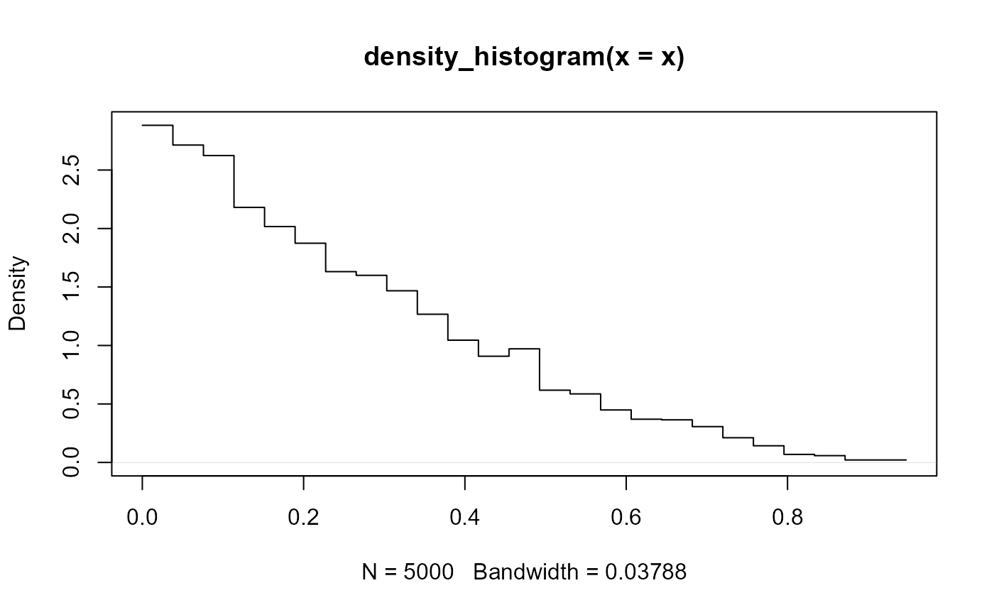
# ... thus, while designed for use with the `density` argument of
# stat_slabinterval(), output from density_histogram() can also be used with
# base::plot():
plot(d)


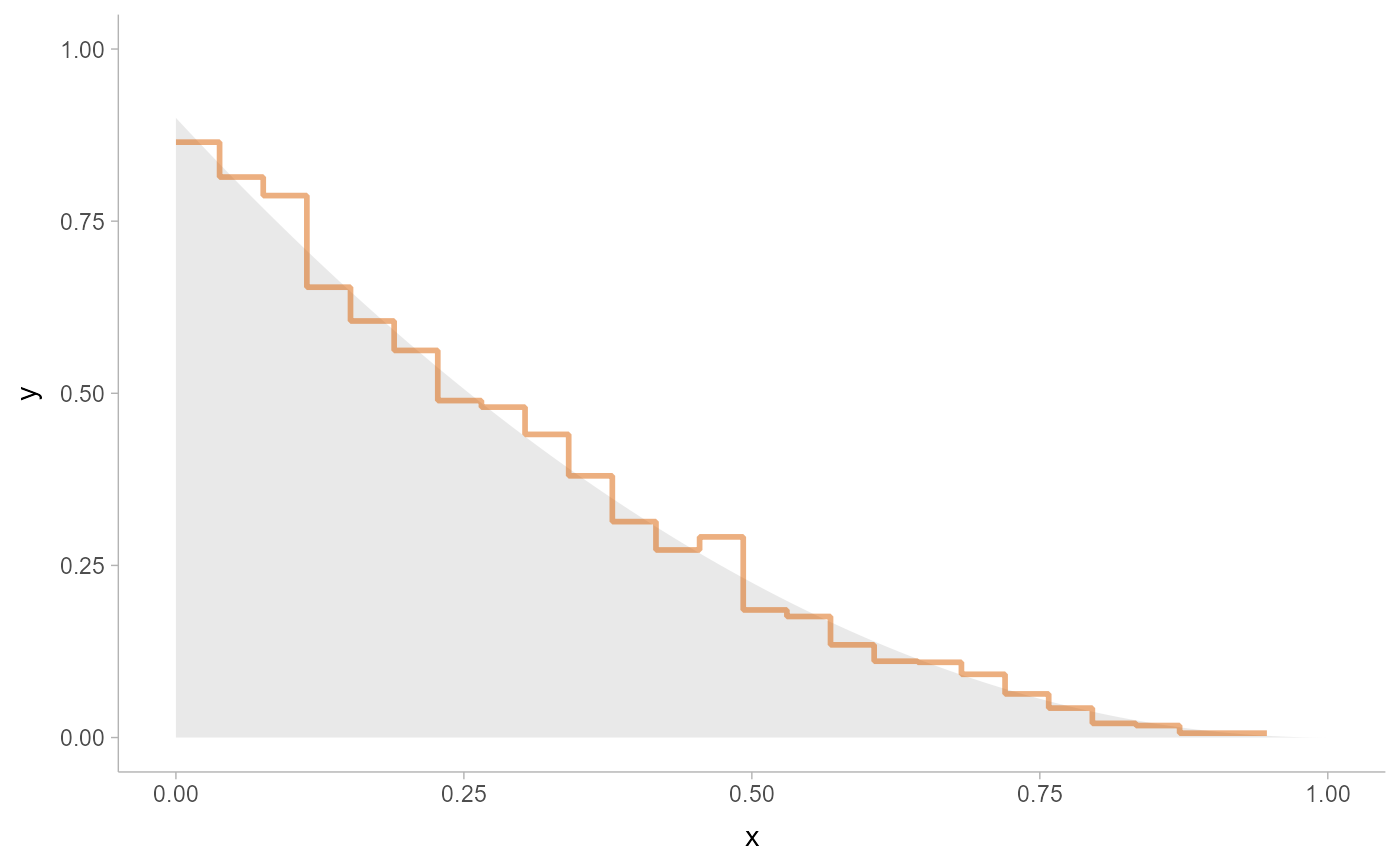
# here we'll use the same data as above with stat_slab():
data.frame(x) %>%
  ggplot() +
  stat_slab(
    aes(xdist = dist), data = data.frame(dist = dist_beta(1, 3)),
    alpha = 0.25
  ) +
  stat_slab(aes(x), density = "histogram", fill = NA, color = "#d95f02", alpha = 0.5) +
  scale_thickness_shared() +
  theme_ggdist()

Usage

Arguments

Value

See also

Examples