Smooth dot positions in a dotplot using a kernel density estimator ("density dotplots")

Smooths x values using a density estimator, returning new x of the same length. Can be used with a dotplot (e.g. geom_dots(smooth = ...)) to create "density dotplots".

Supports automatic partial function application.

Usage

smooth_bounded(
  x,
  density = "bounded",
  bounds = c(NA, NA),
  bounder = "cooke",
  trim = FALSE,
  ...
)

smooth_unbounded(x, density = "unbounded", trim = FALSE, ...)

Arguments

x

a numeric vector

density

Density estimator to use for smoothing. One of:

• A function which takes a numeric vector and returns a list with elements x (giving grid points for the density estimator) and y (the corresponding densities). ggdist provides a family of functions following this format, including density_unbounded() and density_bounded().

• A string giving the suffix of a function name that starts with "density_"; e.g. "bounded" for [density_bounded()].

bounds

length-2 vector of min and max bounds. If a bound is NA, then that bound is estimated from the data using the method specified by bounder.

bounder

Method to use to find missing (NA) bounds. A function that takes a numeric vector of values and returns a length-2 vector of the estimated lower and upper bound of the distribution. Can also be a string giving the suffix of the name of such a function that starts with "bounder_". Useful values include:

• "cdf": Use the CDF of the the minimum and maximum order statistics of the sample to estimate the bounds. See bounder_cdf().

• "cooke": Use the method from Cooke (1979); i.e. method 2.3 from Loh (1984). See bounder_cooke().

• "range": Use the range of x (i.e the min or max). See bounder_range().

trim

Should the density estimate be trimmed to the bounds of the data?

...

Arguments passed to the density estimator specified by density.

Value

A numeric vector of length(x), where each entry is a smoothed version of the corresponding entry in x.

If x is missing, returns a partial application of itself. See automatic-partial-functions.

Details

Applies a kernel density estimator (KDE) to x, then uses weighted quantiles of the KDE to generate a new set of x values with smoothed values. Plotted using a dotplot (e.g. geom_dots(smooth = "bounded") or geom_dots(smooth = smooth_bounded(...)), these values create a variation on a "density dotplot" (Zvinca 2018).

Such plots are recommended only in very large sample sizes where precise positions of individual values are not particularly meaningful. In small samples, normal dotplots should generally be used.

Two variants are supplied by default:

• smooth_bounded(), which uses density_bounded(). Passes the bounds arguments to the estimator.

• smooth_unbounded(), which uses density_unbounded().

It is generally recommended to pick the smooth based on the known bounds of your data, e.g. by using smooth_bounded() with the bounds parameter if there are finite bounds, or smooth_unbounded() if both bounds are infinite.

References

Zvinca, Daniel. "In the pursuit of diversity in data visualization. Jittering data to access details." https://www.linkedin.com/pulse/pursuit-diversity-data-visualization-jittering-access-daniel-zvinca/.

See also

Other dotplot smooths: smooth_discrete(), smooth_none()

Examples

library(ggplot2)

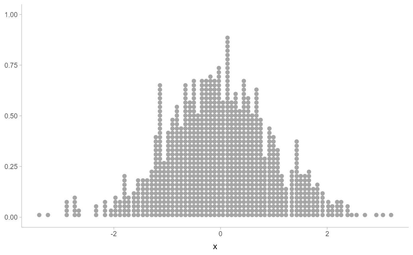
set.seed(1234)
x = rnorm(1000)

# basic dotplot is noisy
ggplot(data.frame(x), aes(x)) +
  geom_dots()


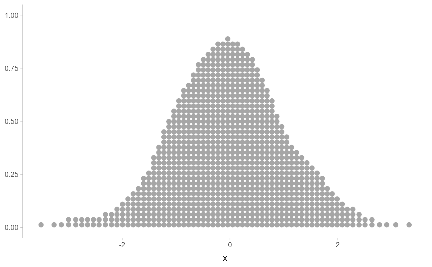
# density dotplot is smoother, but does move points (most noticeable
# in areas of low density)
ggplot(data.frame(x), aes(x)) +
  geom_dots(smooth = "unbounded")


# you can adjust the kernel and bandwidth...
ggplot(data.frame(x), aes(x)) +
  geom_dots(smooth = smooth_unbounded(kernel = "triangular", adjust = 0.5))


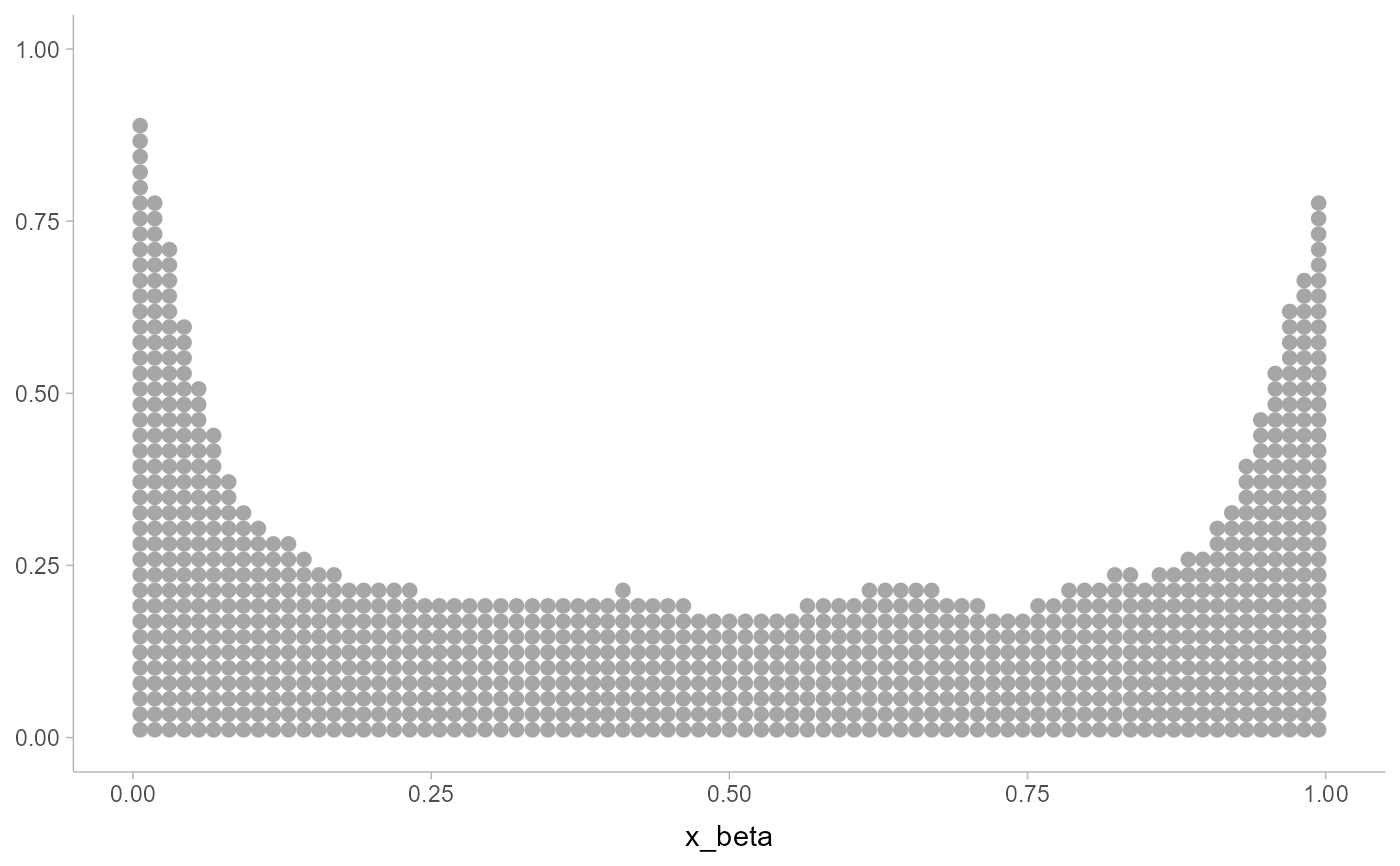
# for bounded data, you should use the bounded smoother
x_beta = rbeta(1000, 0.5, 0.5)

ggplot(data.frame(x_beta), aes(x_beta)) +
  geom_dots(smooth = smooth_bounded(bounds = c(0, 1)))