Slab thickness scale (ggplot2 scale)

This ggplot2 scale linearly scales all thickness values of geoms that support the thickness aesthetic (such as geom_slabinterval()). It can be used to align the thickness scales across multiple geoms (by default, thickness is normalized on a per-geom level instead of as a global scale). For a comprehensive discussion and examples of slab scaling and normalization, see the thickness scale article.

Usage

scale_thickness_shared(
  name = waiver(),
  breaks = waiver(),
  labels = waiver(),
  limits = function(l) c(min(0, l[[1]]), l[[2]]),
  renormalize = FALSE,
  oob = scales::oob_keep,
  guide = "none",
  ...
)

scale_thickness_identity(..., guide = "none")

thickness(x = double(), lower = NA_real_, upper = NA_real_)

Arguments

name

The name of the scale. Used as the axis or legend title. If waiver(), the default, the name of the scale is taken from the first mapping used for that aesthetic. If NULL, the legend title will be omitted.

breaks

One of:

• NULL for no breaks

• waiver() for the default breaks computed by the transformation object

• A numeric vector of positions

• A function that takes the limits as input and returns breaks as output (e.g., a function returned by scales::extended_breaks()). Also accepts rlang lambda function notation.

labels

One of:

• NULL for no labels

• waiver() for the default labels computed by the transformation object

• A character vector giving labels (must be same length as breaks)

• An expression vector (must be the same length as breaks). See ?plotmath for details.

• A function that takes the breaks as input and returns labels as output. Also accepts rlang lambda function notation.

limits

One of:

• NULL to use the default scale range

• A numeric vector of length two providing limits of the scale. Use NA to refer to the existing minimum or maximum

• A function that accepts the existing (automatic) limits and returns new limits. Also accepts rlang lambda function notation. Note that setting limits on positional scales will remove data outside of the limits. If the purpose is to zoom, use the limit argument in the coordinate system (see coord_cartesian()).

renormalize

When mapping values to the thickness scale, should those values be allowed to be renormalized by geoms (e.g. via the normalize parameter to geom_slabinterval())? The default is FALSE: if scale_thickness_shared() is in use, the geom-specific normalize parameter is ignored (this is achieved by flagging values as already normalized by wrapping them in thickness()). Set this to TRUE to allow geoms to also apply their own normalization. Note that if you set renormalize to TRUE, subguides created via the subguide parameter to geom_slabinterval() will display the scaled values output by this scale, not the original data values.

oob

One of:

• Function that handles limits outside of the scale limits (out of bounds). Also accepts rlang lambda function notation.

• The default (scales::censor()) replaces out of bounds values with NA.

• scales::squish() for squishing out of bounds values into range.

• scales::squish_infinite() for squishing infinite values into range.

guide

A function used to create a guide or its name. See guides() for more information.

...

Arguments passed on to ggplot2::continuous_scale

aesthetics

The names of the aesthetics that this scale works with.

scale_name

The name of the scale that should be used for error messages associated with this scale.

palette

A palette function that when called with a numeric vector with values between 0 and 1 returns the corresponding output values (e.g., scales::pal_area()).

minor_breaks

One of:

• NULL for no minor breaks

• waiver() for the default breaks (one minor break between each major break)

• A numeric vector of positions

• A function that given the limits returns a vector of minor breaks. Also accepts rlang lambda function notation. When the function has two arguments, it will be given the limits and major breaks.

n.breaks

An integer guiding the number of major breaks. The algorithm may choose a slightly different number to ensure nice break labels. Will only have an effect if breaks = waiver(). Use NULL to use the default number of breaks given by the transformation.

rescaler

A function used to scale the input values to the range [0, 1]. This is always scales::rescale(), except for diverging and n colour gradients (i.e., scale_colour_gradient2(), scale_colour_gradientn()). The rescaler is ignored by position scales, which always use scales::rescale(). Also accepts rlang lambda function notation.

expand

For position scales, a vector of range expansion constants used to add some padding around the data to ensure that they are placed some distance away from the axes. Use the convenience function expansion() to generate the values for the expand argument. The defaults are to expand the scale by 5% on each side for continuous variables, and by 0.6 units on each side for discrete variables.

na.value

Missing values will be replaced with this value.

transform

For continuous scales, the name of a transformation object or the object itself. Built-in transformations include "asn", "atanh", "boxcox", "date", "exp", "hms", "identity", "log", "log10", "log1p", "log2", "logit", "modulus", "probability", "probit", "pseudo_log", "reciprocal", "reverse", "sqrt" and "time".

A transformation object bundles together a transform, its inverse, and methods for generating breaks and labels. Transformation objects are defined in the scales package, and are called transform_<name>. If transformations require arguments, you can call them from the scales package, e.g. scales::transform_boxcox(p = 2). You can create your own transformation with scales::new_transform().

trans

Deprecated in favour of transform.

position

For position scales, The position of the axis. left or right for y axes, top or bottom for x axes.

call

The call used to construct the scale for reporting messages.

super

The super class to use for the constructed scale

x

An object (typically a numeric()) to be converted to a thickness() object.

lower

The original lower bounds of thickness values before scaling.

upper

The original upper bounds of thickness values before scaling.

Value

A ggplot2::Scale representing a scale for the thickness

aesthetic for ggdist geoms. Can be added to a ggplot() object.

Details

By default, normalization/scaling of slab thicknesses is controlled by geometries, not by a ggplot2 scale function. This allows various functionality not otherwise possible, such as (1) allowing different geometries to have different thickness scales and (2) allowing the user to control at what level of aggregation (panels, groups, the entire plot, etc) thickness scaling is done via the normalize parameter to geom_slabinterval().

However, this default approach has one drawback: two different geoms will always have their own scaling of thickness. scale_thickness_shared() offers an alternative approach: when added to a chart, all geoms will use the same thickness scale, and geom-level normalization (via their normalize parameters) is ignored. This is achieved by "marking" thickness values as already normalized by wrapping them in the thickness() data type (this can be disabled by setting renormalize = TRUE).

thickness() is used by scale_thickness_shared() to create numeric()-like objects marked as being in units of slab "thickness". Unlike regular numeric()s, thickness() values mapped onto the thickness aesthetic are not rescaled by scale_thickness_shared() or geom_slabinterval(). In most cases thickness() is not useful directly; though it can be used to mark values that should not be rescaled---see the definitions of stat_ccdfinterval() and stat_gradientinterval() for some usages.

Note: while a slightly more typical name for scale_thickness_shared() might be scale_thickness_continuous(), the latter name would cause this scale to be applied to all thickness aesthetics by default according to the rules ggplot2 uses to find default scales. Thus, to retain the usual behavior of stat_slabinterval() (per-geom normalization of thickness), this scale is called scale_thickness_shared().

See also

The thickness aesthetic of geom_slabinterval().

Other ggdist scales: scale_colour_ramp, scale_side_mirrored(), sub-geometry-scales

Author

Matthew Kay

Examples

library(distributional)
library(ggplot2)
library(dplyr)

prior_post = data.frame(
  prior = dist_normal(0, 1),
  posterior = dist_normal(0.1, 0.5)
)

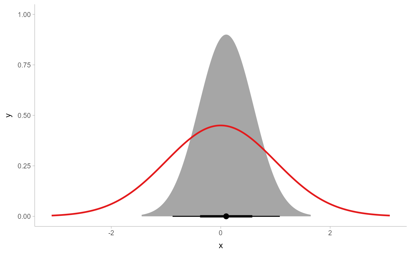
# By default, separate geoms have their own thickness scales, which means
# distributions plotted using two separate geoms will not have their slab
# functions drawn on the same scale (thus here, the two distributions have
# different areas under their density curves):
prior_post %>%
  ggplot() +
  stat_halfeye(aes(xdist = posterior)) +
  stat_slab(aes(xdist = prior), fill = NA, color = "red")


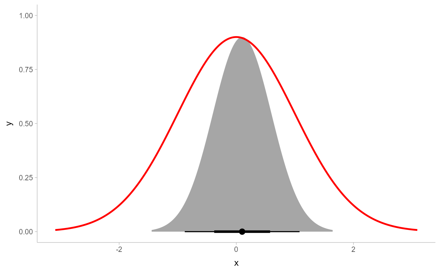# For this kind of prior/posterior chart, it makes more sense to have the
# densities on the same scale; thus, the areas under both would be the same.
# We can do that using scale_thickness_shared():
prior_post %>%
  ggplot() +
  stat_halfeye(aes(xdist = posterior)) +
  stat_slab(aes(xdist = prior), fill = NA, color = "#e41a1c") +
  scale_thickness_shared()