Bounded density estimator using the reflection method

Bounded density estimator using the reflection method.

Supports automatic partial function application.

Usage

density_bounded(
  x,
  weights = NULL,
  n = 512,
  bandwidth = "dpi",
  adjust = 1,
  kernel = "gaussian",
  trim = FALSE,
  bounds = c(NA, NA),
  bounder = "cdf",
  adapt = 1,
  na.rm = FALSE,
  ...,
  range_only = FALSE
)

Arguments

x

numeric vector containing a sample to compute a density estimate for.

weights

optional numeric vector of weights to apply to x.

n

numeric: the number of grid points to evaluate the density estimator at.

bandwidth

bandwidth of the density estimator. One of:

a numeric: the bandwidth, as the standard deviation of the kernel
a function: a function taking x (the sample) and returning the bandwidth
a string: the suffix of the name of a function starting with "bandwidth_" that will be used to determine the bandwidth. See bandwidth for a list.

adjust

numeric: the bandwidth for the density estimator is multiplied by this value. See stats::density().

kernel

string: the smoothing kernel to be used. This must partially match one of "gaussian", "rectangular", "triangular", "epanechnikov", "biweight", "cosine", or "optcosine". See stats::density().

trim

Should the density estimate be trimmed to the bounds of the data?

bounds

length-2 vector of min and max bounds. If a bound is NA, then that bound is estimated from the data using the method specified by bounder.

bounder

Method to use to find missing (NA) bounds. A function that takes a numeric vector of values and returns a length-2 vector of the estimated lower and upper bound of the distribution. Can also be a string giving the suffix of the name of such a function that starts with "bounder_". Useful values include:

"cdf": Use the CDF of the the minimum and maximum order statistics of the sample to estimate the bounds. See bounder_cdf().
"cooke": Use the method from Cooke (1979); i.e. method 2.3 from Loh (1984). See bounder_cooke().
"range": Use the range of x (i.e the min or max). See bounder_range().

adapt

(very experimental) The name and interpretation of this argument are subject to change without notice. Positive integer. If adapt > 1, uses an adaptive approach to calculate the density. First, uses the adaptive bandwidth algorithm of Abramson (1982) to determine local (pointwise) bandwidths, then groups these bandwidths into adapt groups, then calculates and sums the densities from each group. You can set this to a very large number (e.g. Inf) for a fully adaptive approach, but this will be very slow; typically something around 100 yields nearly identical results.

na.rm

Should missing (NA) values in x be removed?

...

Additional arguments (ignored).

range_only

If TRUE, the range of the output of this density estimator is computed and is returned in the $x element of the result, and c(NA, NA) is returned in $y. This gives a faster way to determine the range of the output than density_XXX(n = 2).

Value

An object of class "density", mimicking the output format of stats::density(), with the following components:

x: The grid of points at which the density was estimated.
y: The estimated density values.
bw: The bandwidth.
n: The sample size of the x input argument.
call: The call used to produce the result, as a quoted expression.
data.name: The deparsed name of the x input argument.
has.na: Always FALSE (for compatibility).
cdf: Values of the (possibly weighted) empirical cumulative distribution function at x. See weighted_ecdf().

This allows existing methods for density objects, like print() and plot(), to work if desired. This output format (and in particular, the x and y components) is also the format expected by the density argument of the stat_slabinterval()

and the smooth_ family of functions.

References

Cooke, P. (1979). Statistical inference for bounds of random variables. Biometrika 66(2), 367--374. doi:10.1093/biomet/66.2.367 .

Loh, W. Y. (1984). Estimating an endpoint of a distribution with resampling methods. The Annals of Statistics 12(4), 1543--1550. doi:10.1214/aos/1176346811

Examples

library(distributional)
library(dplyr)
library(ggplot2)

# For compatibility with existing code, the return type of density_bounded()
# is the same as stats::density(), ...
set.seed(123)
x = rbeta(5000, 1, 3)
d = density_bounded(x)
d
#> 
#> Call:
#> 	density_bounded(x = x)
#> 
#> Data: x (5000 obs.);	Bandwidth 'bw' = 0.01647
#> 
#>        x                    y            
#>  Min.   :-0.0001229   Min.   :0.0009348  
#>  1st Qu.: 0.2467302   1st Qu.:0.2144899  
#>  Median : 0.4935833   Median :0.8152210  
#>  Mean   : 0.4935833   Mean   :1.0138543  
#>  3rd Qu.: 0.7404364   3rd Qu.:1.6212908  
#>  Max.   : 0.9872895   Max.   :2.9045616  

# ... thus, while designed for use with the `density` argument of
# stat_slabinterval(), output from density_bounded() can also be used with
# base::plot():
plot(d)


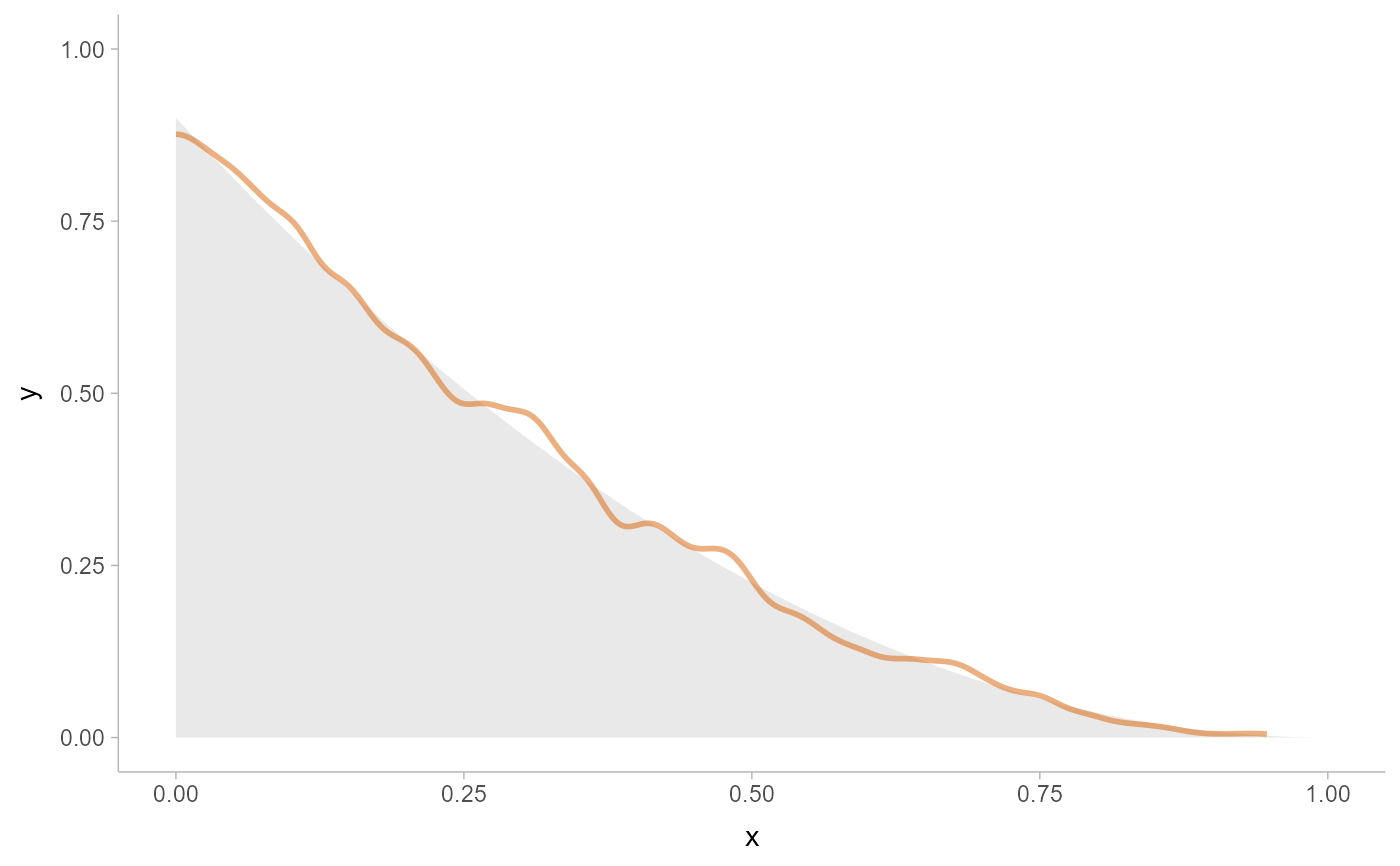
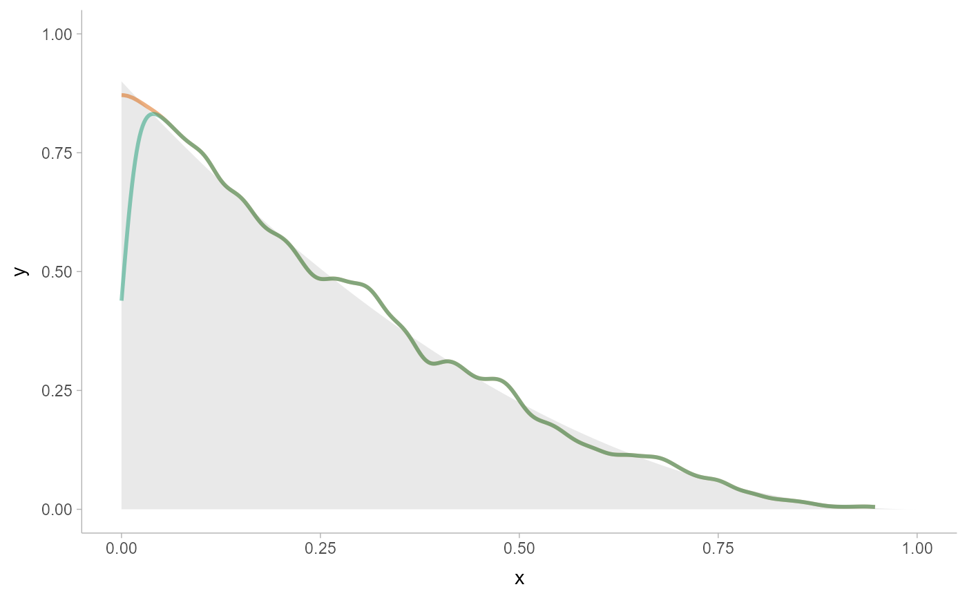
# here we'll use the same data as above, but pick either density_bounded()
# or density_unbounded() (which is equivalent to stats::density()). Notice
# how the bounded density (green) is biased near the boundary of the support,
# while the unbounded density is not.
data.frame(x) %>%
  ggplot() +
  stat_slab(
    aes(xdist = dist), data = data.frame(dist = dist_beta(1, 3)),
    alpha = 0.25
  ) +
  stat_slab(aes(x), density = "bounded", fill = NA, color = "#d95f02", alpha = 0.5) +
  stat_slab(aes(x), density = "unbounded", fill = NA, color = "#1b9e77", alpha = 0.5) +
  scale_thickness_shared() +
  theme_ggdist()


# We can also supply arguments to the density estimators by using their
# full function names instead of the string suffix; e.g. we can supply
# the exact bounds of c(0,1) rather than using the bounds of the data.
data.frame(x) %>%
  ggplot() +
  stat_slab(
    aes(xdist = dist), data = data.frame(dist = dist_beta(1, 3)),
    alpha = 0.25
  ) +
  stat_slab(
    aes(x), fill = NA, color = "#d95f02", alpha = 0.5,
    density = density_bounded(bounds = c(0,1))
  ) +
  scale_thickness_shared() +
  theme_ggdist()