Thickness scale

Introduction

This vignette describes the thickness scale / aesthetic used by the slab+interval family of geoms and stats in ggdist (see vignette("slabinterval") for more on that family).

Setup

The following libraries are required to run this vignette:

library(ggplot2)
library(dplyr)
library(distributional)
library(ggdist)

theme_set(theme_ggdist())

The `thickness` scale

The thickness scale is a positional subscale used by geom_slabinterval() to construct slabs, which are ribbon-like geometries with a fixed baseline and a height determined by the thickness aesthetic. The thickness scale is most typically used via stat_slabinterval() and its derivative stats, which allow you to map distribution functions (like densities or CDFs) onto the thickness aesthetic.

thickness exists as a scale separate from the typical x and y aesthetics (or even width/height, xmin/xmax, or ymin/ymax) so that it is easy to plot multiple slabs on the same plot, each with its own separate thickness subscale. For example:

df = tibble(
  h = c(0,1,1,0, 0,2,2,0, 0,4/3,4/3,0,  0,1,1,0,     0,1.25,1.25,0, 0,.5,.5,0),
  x = c(0,1,4,5, 4,5,6,7, 6,7,9,10,     11,12,15,16, 1,2,4.2,5.2,   4,5,12,13),
  y     = rep(c("a", "b", "a", "a", "b", "a"), each = 4),
  group = rep(c("c", "c", "d", "d", "c", "c"), each = 4),
  panel = rep(c("e", "e", "e", "e", "f", "f"), each = 4),
  name  = rep(c(1,    2, "3a","3b",  4,   5),  each = 4)
)

df_group = df %>%
  summarise(x = mean(x), .by = c(name, group, panel, y))

df %>%
  ggplot(aes(x = x, y = y, fill = group, thickness = h)) +
  geom_slab(color = "gray25", alpha = 0.75) +
  scale_y_discrete(expand = expansion(add = 0.1)) +
  scale_fill_brewer(palette = "Set2") +
  facet_grid(cols = vars(panel), labeller = "label_both") +
  labs("geom_slab() with default thickness scaling") +
  theme(
    legend.position = "bottom",
    panel.grid.major.y = element_line(color = "gray85"),
    panel.background = element_rect(color = "gray70", fill = NA)
  )

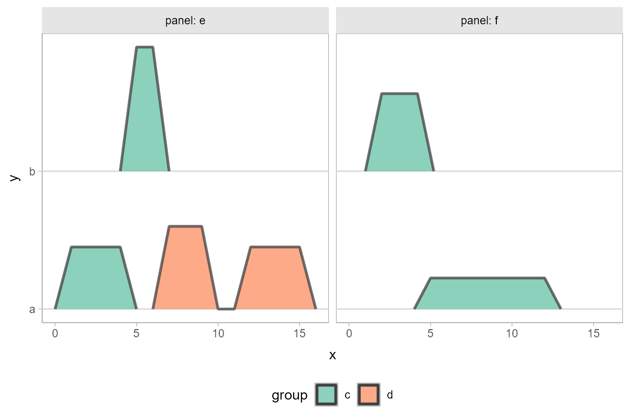
In the above plot, the values assigned to the thickness aesthetic are all scaled onto a common scale, and the slabs are positioned with their baselines at the y value specified for each slab.

Adjusting normalization within one geometry

The default thickness scaling shown above corresponds to the normalize = "all" option of geom_slab(). It uses the same scale for all slabs, scaling them according the the maximum height of the tallest slab.

The normalize parameter provides a set of options that define a hierarchy of increasingly more specific sets within which to scale the slabs:

"all" scales according to the maximum over all slabs;
"panels" scales according to the maximum within each panel (facet);
"xy" scales according to the maximum within each x/y position within each panel; and
"groups" scales according to the maximum within each group within each x/y position within each panel.

The x/y position referred to above is the unique x or y position of the slab on its off-axis. For example, this would be the unique y positions in the above chart ("a" or "b"), because the chart is drawn with a horizontal orientation.

`normalize = "all"`

We can see how normalization affects the scales by annotating the previous plot of the default normalization settings:

subguide_orangered = subguide_outside(
  title = "thickness",
  position = "right",
  theme = theme_ggdist() + theme(
    text = element_text(color = "orangered"),
    axis.line.y = element_line(color = "orangered"),
    axis.ticks.y = element_line(color = "orangered"),
    axis.text.y = element_text(color = "orangered")
  )
)

plot_slabs_with_scales = function(..., subguide = subguide_orangered) {
  df %>%
    ggplot(aes(x = x, y = y, fill = group)) +
    geom_hline(yintercept = c(1,1.9, 2,2.9), color = "orangered", linetype = "11", linewidth = 0.5) +
    geom_slab(
      aes(thickness = h),
      subguide = subguide,
      alpha = 0.75,
      color = "gray25",
      ...
    ) +
    geom_label(
      aes(label = name),
      data = df_group,
      color = "gray25",
      alpha = 0.75,
      vjust = 0,
      show.legend = FALSE
    ) +
    scale_y_discrete(expand = expansion(add = 0.1)) +
    scale_fill_brewer(palette = "Set2") +
    facet_grid(cols = vars(panel), labeller = "label_both") +
    theme(
      plot.margin = margin(5.5, 50, 5.5, 5.5),
      panel.spacing.x = unit(40, "pt"),
      legend.position = "bottom",
      panel.background = element_rect(color = "gray70", fill = NA)
    )
}

plot_slabs_with_scales(normalize = "all") +
  labs(
    title = "geom_slab(normalize = 'all')",
    subtitle = "default normalization settings"
  )

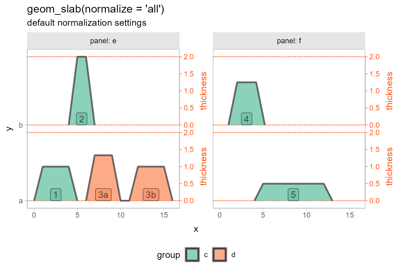
Notice how the minimum and maximum value on each thickness subscale is the same: it is the maximum thickness value over all slabs; i.e. the height of the tallest slab in the data. This is a conservative default setting that ensures all slabs in the same geometry are scaled together.

`normalize = "panels"`

Sometimes you may have separate panels within which you want to scale all slabs together. You can do this using normalize = "panels":

plot_slabs_with_scales(normalize = "panels") +
  labs(
    title = "geom_slab(normalize = 'panels')",
    subtitle = "scales to the maximum height within each panel"
  )

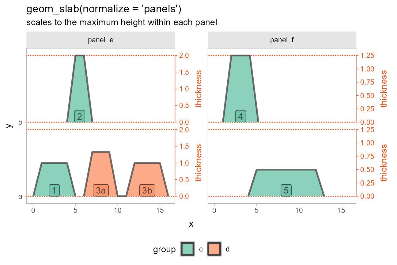
Notice how the thickness scales inside a given panel are the same: panel "e" has a maximum thickness of 2 (the height of slab 2) and panel "f" has a maximum thickness of 1.25 (the height of slab 4). All other slabs within the same panel are scaled accordingly.

`normalize = "xy"`

Often it is useful to scale slabs on the same x or y position together, where whether we scale within x or y is determined by the orientation of the geometry. You can do this using normalize = "xy":

plot_slabs_with_scales(normalize = "xy") +
  labs(
    title = "geom_slab(normalize = 'xy')",
    subtitle = "scales to the maximum height within each x/y position within each panel"
  )

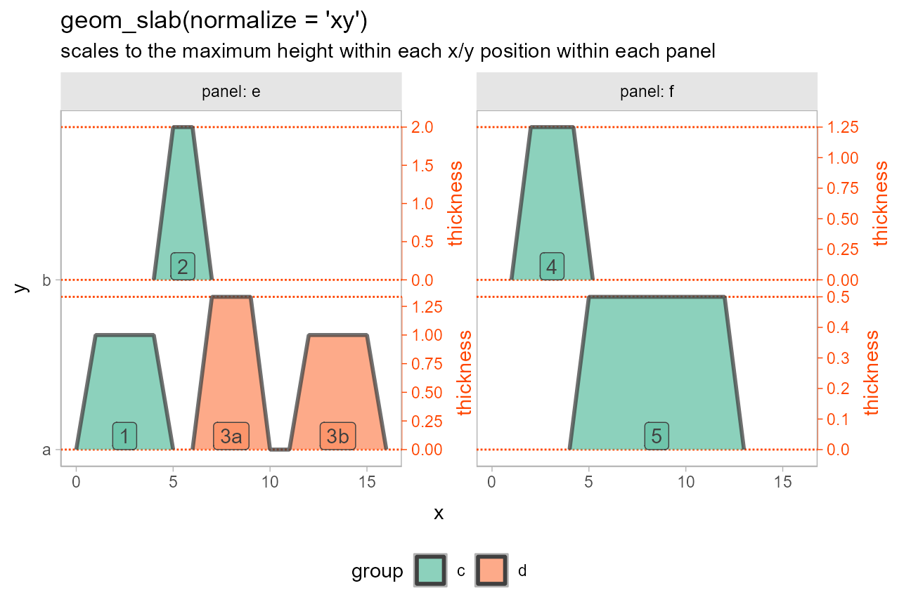
In this plot, because orientation = "horizontal", normalize = "xy" scales within each unique y position; i.e. the values "a" and "b". Normalization settings are hierarchical, so it uses the maximum thickness value within each y position within each panel. Thus:

slab 2 is scaled to its maximum of 2.0;
slabs 1, 3a, and 3b are scaled to their maximum of 1.33 (the height of slab 3a);
slab 4 is scaled to its maximum of 1.25; and
slab 5 is scaled to its maximum of 0.5.

`normalize = "groups"`

Finally, it can be useful to scale all slabs according to their maximum height. You can do this using normalize = "groups".

Notably, if you have multiple groups at the same x/y position, you cannot combine normalize = "groups" with any thickness subguide except "none", because the thickness subguides on each y value will not be unique. Hence this error:

plot_slabs_with_scales(normalize = "groups")

## Error in `geom_slab()`:
## ! Problem while converting geom to grob.
## ℹ Error occurred in the 2nd layer.
## Caused by error in `fun()`:
## ! Cannot draw a subguide for the thickness axis when multiple slabs with different
##   normalizations are drawn on the same axis.

Thus for this example we will have to omit the thickness subguide:

plot_slabs_with_scales(normalize = "groups", subguide = "none") +
  labs(
    title = "geom_slab(normalize = 'groups')",
    subtitle = "scales to the maximum height within each group within each x/y position within each panel"
  )

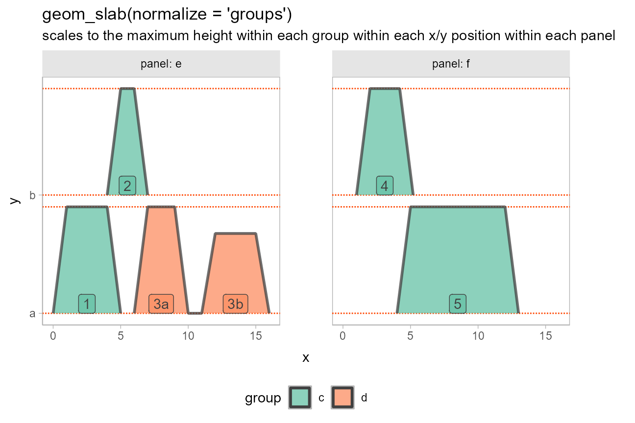
Notice how all groups are scaled to have their maximum height at the maximum thickness value; thus, slab 1 and slab 3b are no longer the same height.

Why is slab 3b not scaled to touch the maximum thickness? geom_slab() technically only considers values in different groups to be in different slabs, so slab 3a and 3b are actually parts of the same slab, as indicated by the unbroken outline they are drawn with.

Sharing `thickness` scales across multiple geometries

Sometimes we want to use different geometries to plot slabs on the same scale. This often happens when plotting priors and posteriors, but may happen in other cases as well.

Here is a prior and posterior plotted using separate geometries, with their thickness scales annotated:

df_prior_post = data.frame(
  prior = dist_normal(0, 1),
  posterior = dist_normal(0.1, 0.3)
)

prior_post_plot = df_prior_post %>%
  ggplot() +
  stat_slab(
    aes(xdist = posterior),
    subguide = subguide_inside(title = "posterior thickness")
  ) +
  stat_slab(
    aes(xdist = prior),
    color = "orangered",
    fill = NA,
    subguide = subguide_orangered(title = "prior thickness", just = 0, label_side = "inside")
  ) +
  scale_y_continuous(breaks = NULL) +
  theme(panel.background = element_rect(color = "gray70", fill = NA))

prior_post_plot +
  labs(
    title = "two different slab geometries",
    subtitle = "thickness scales are not shared across geometries by default"
  )

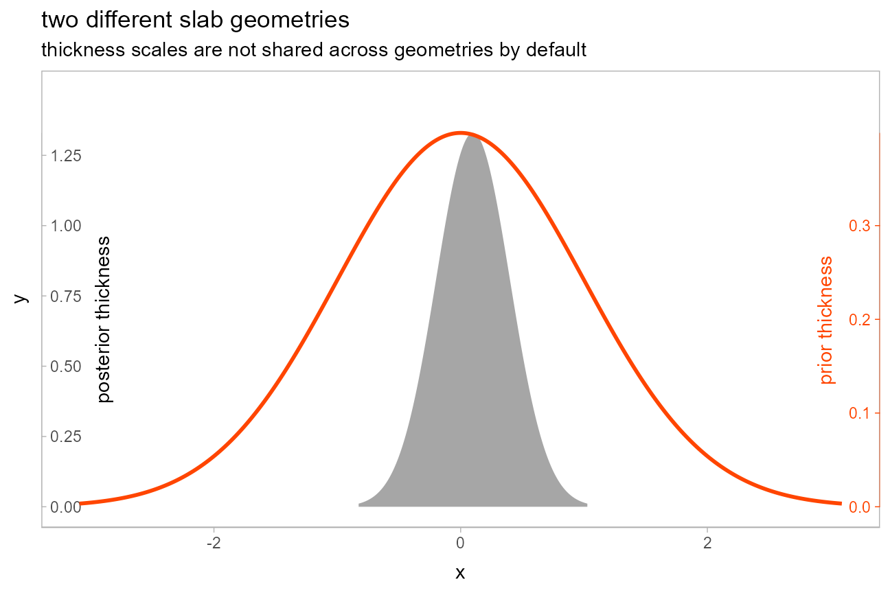
Notice how the two geometries have different thickness scales. If we add scale_thickness_shared() to the plot, they will be given the same scale:

prior_post_plot +
  scale_thickness_shared() +
  labs(
    title = "two different slab geometries",
    subtitle = "using scale_thickness_shared() to share thickness scale across geometries"
  )

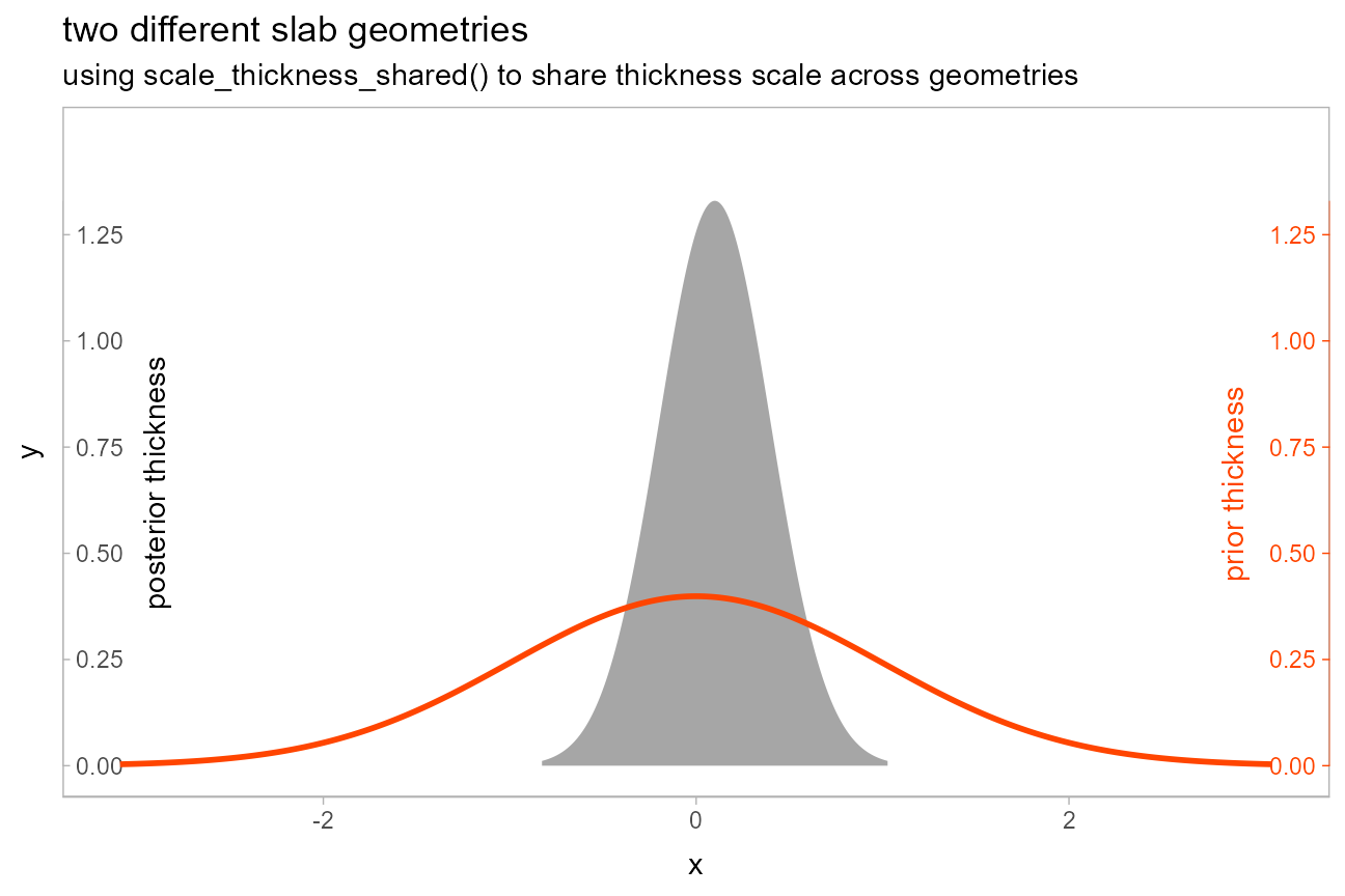
scaled_thickness_shared() works by scaling values and then tagging them with a special thickness() datatype. That type carries information about the original scale limits (used to draw subguides), and also tells the slab geometries that they should not do any further normalization. Thus, when you use scale_thickness_shared(), the normalize parameter on each slab geometry is ignored.

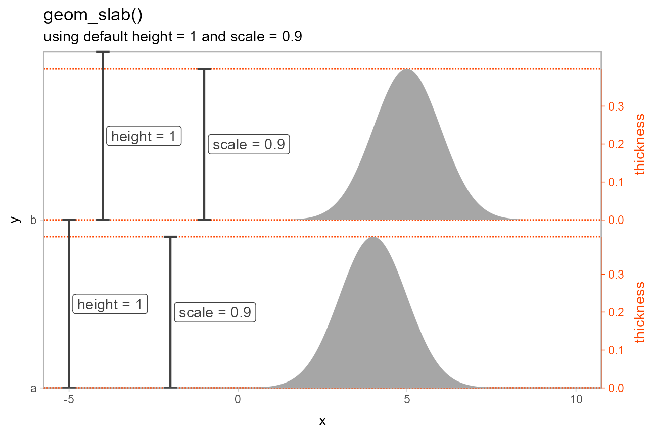
Spacing slabs with `height` and `scale`

The thickness aesthetic is drawn within a subset of the bounding box of geom_slab() determined by the scale aesthetic, which defaults to 0.9:

cap = arrow(angle = 90, length = unit(5, "pt"), ends = "both")

scale_plot = function(scale = 0.9) {
  tibble(d = dist_normal(c(4,5)), y = c("a","b")) %>%
    ggplot(aes(xdist = d, y = y)) +
    geom_hline(
      yintercept = c(1, 1 + scale, 2, 2 + scale),
      color = "orangered", linetype = "11", linewidth = 0.5
    ) +
    stat_slab(scale = scale, subguide = subguide_orangered) +
    annotate("segment", x = c(-5,-4), xend = c(-5,-4), y = c(1,2), yend = c(2,3),
      arrow = cap, linewidth = 0.75, color = "gray25"
    ) +
    annotate("label", x = c(-5,-4), y = c(1.5, 2.5),
      label = "height = 1", hjust = -0.05, color = "gray25"
    ) +
    annotate("segment", x = c(-2,-1), xend = c(-2,-1), y = c(1,2), yend = c(1,2) + scale,
      arrow = cap, linewidth = 0.75, color = "gray25"
    ) +
    annotate("label", x = c(-2,-1), y = c(1,2) + scale/2,
      label = paste("scale =", scale), hjust = -0.05, color = "gray25"
    ) +
    scale_y_discrete(expand = expansion(add = 0)) +
    scale_x_continuous(limits = c(-5, 10)) +
    theme(
      plot.margin = margin(5.5, 40, 5.5, 5.5),
      panel.background = element_rect(color = "gray70")
    ) +
    coord_cartesian(clip = "off")
}

scale_plot(scale = 0.9) +
  labs(
    title = "geom_slab()",
    subtitle = "using default height = 1 and scale = 0.9"
  )

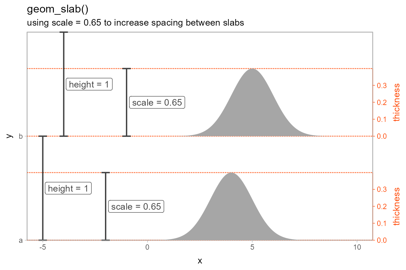
This allows us to adjust the spacing between slabs using scale:

scale_plot(scale = 0.65) +
  labs(
    title = "geom_slab()",
    subtitle = "using scale = 0.65 to increase spacing between slabs"
  )

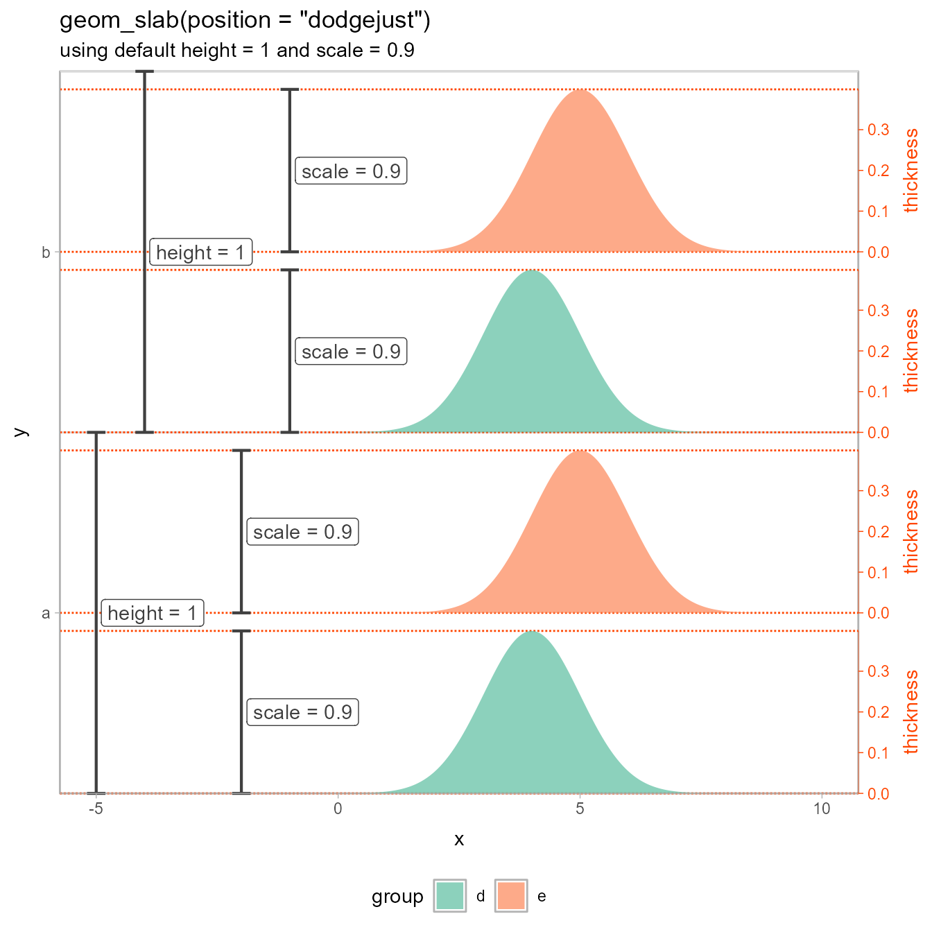
Spacing dodged slabs

height and scale are particularly useful when combined with dodging, as modifying height allows you to change the spacing between sets of slabs with the same y value, and modifying scale allows you to change the spacing within sets:

dodged_scale_plot = function(height = 1, scale = 0.9, add = 0) {
  baselines = c(1 - height/2, 1, 2 - height/2, 2)
  tibble(
    d = dist_normal(c(4,5,4,5)),
    y = c("a","a","b","b"),
    group = c("d","e","d","e")
  ) %>%
    ggplot(aes(xdist = d, y = y, fill = group)) +
    geom_hline(yintercept = c(1,2) + height/2, color = "gray85") +
    geom_hline(
      yintercept = c(baselines, baselines + height/2*scale),
      color = "orangered",
      linetype = "11",
      linewidth = 0.5
    ) +
    stat_slab(
      height = height, scale = scale,
      subguide = subguide_orangered, position = "dodgejust",
      alpha = 0.75
    ) +
    annotate("segment",
      x = c(-5,-4), xend = c(-5,-4),
      y = c(1,2) - height/2, yend = c(1,2) + height/2,
      arrow = cap, color = "gray25", linewidth = 0.75
    ) +
    annotate("label", x = c(-5,-4), y = c(1, 2),
      label = paste("height =", height), hjust = -0.05,
      color = "gray25"
    ) +
    annotate("segment", x = c(-2,-2,-1,-1), xend = c(-2,-2,-1,-1),
      y = baselines, yend = baselines + scale * height/2,
      arrow = cap, color = "gray25", linewidth = 0.75
    ) +
    annotate("label", x = c(-2,-2,-1,-1),
      y = baselines + scale*height/4, label = paste("scale =", scale),
      hjust = -0.05, color = "gray25"
    ) +
    scale_y_discrete(expand = expansion(add = add)) +
    scale_x_continuous(limits = c(-5, 10)) +
    scale_fill_brewer(palette = "Set2") +
    theme(
      plot.margin = margin(5.5, 40, 5.5, 5.5),
      panel.background = element_rect(color = "gray70"),
      legend.position = "bottom"
    ) +
    coord_cartesian(clip = "off")
}

dodged_scale_plot(height = 1, scale = 0.9, add = 0) +
  labs(
    title = 'geom_slab(position = "dodgejust")',
    subtitle = "using default height = 1 and scale = 0.9"
  )

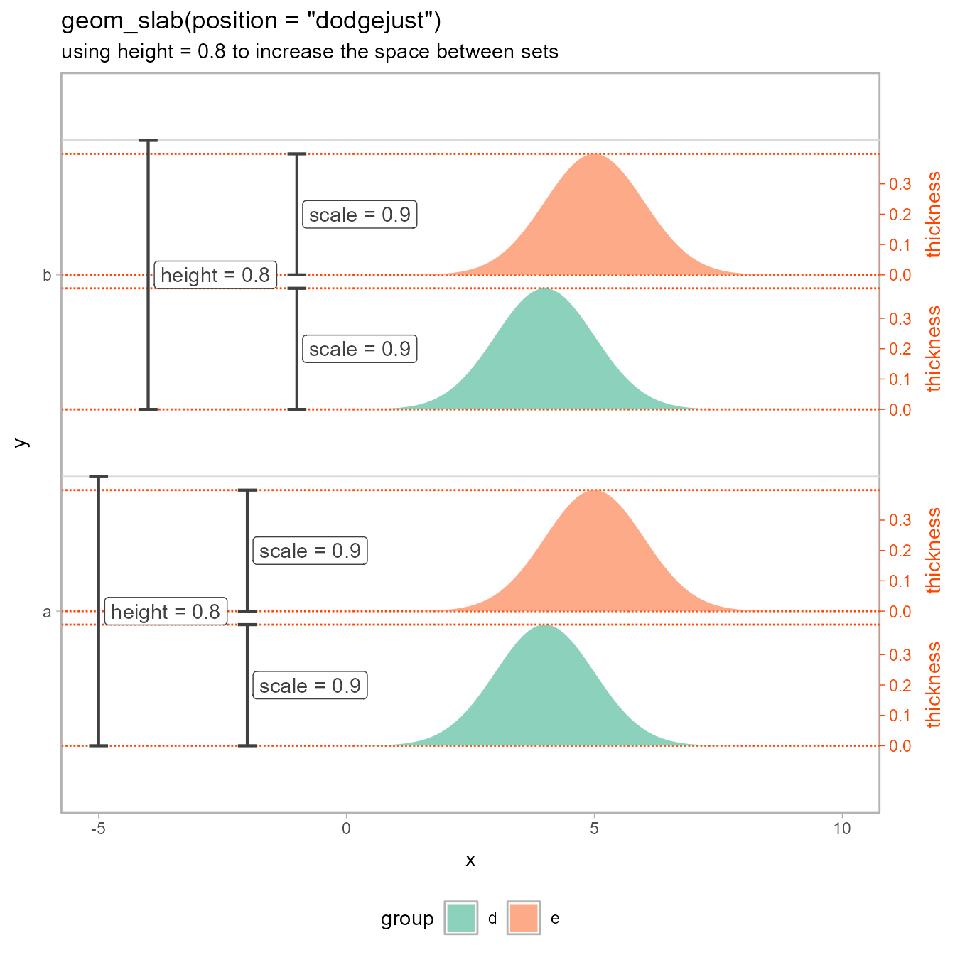
If we decrease height, it increases the space between sets of slabs with the same y value:

dodged_scale_plot(height = 0.8, scale = 0.9, add = 0.6) +
  labs(
    title = 'geom_slab(position = "dodgejust")',
    subtitle = "using height = 0.8 to increase the space between sets"
  )

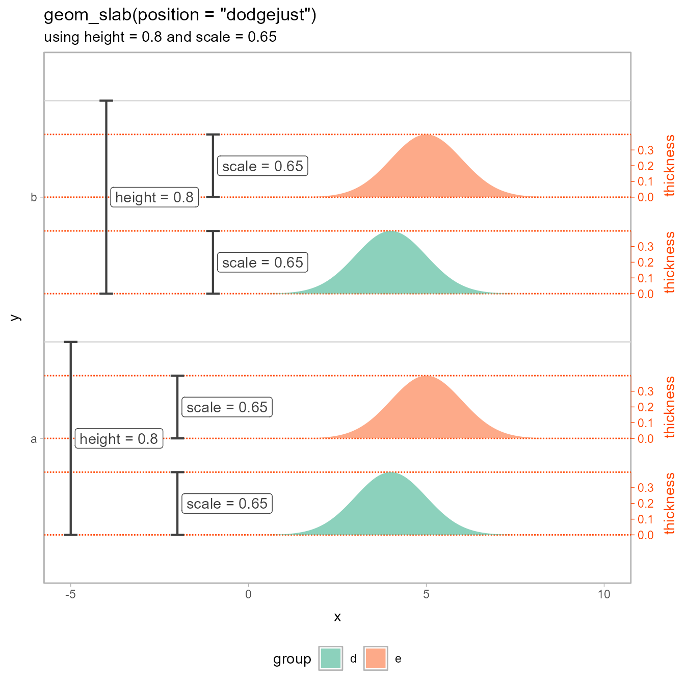
And if we decrease scale, it increases the spacing within sets of slabs with the same y value:

dodged_scale_plot(height = 0.8, scale = 0.65, add = 0.6) +
  labs(
    title = 'geom_slab(position = "dodgejust")',
    subtitle = "using height = 0.8 and scale = 0.65"
  )

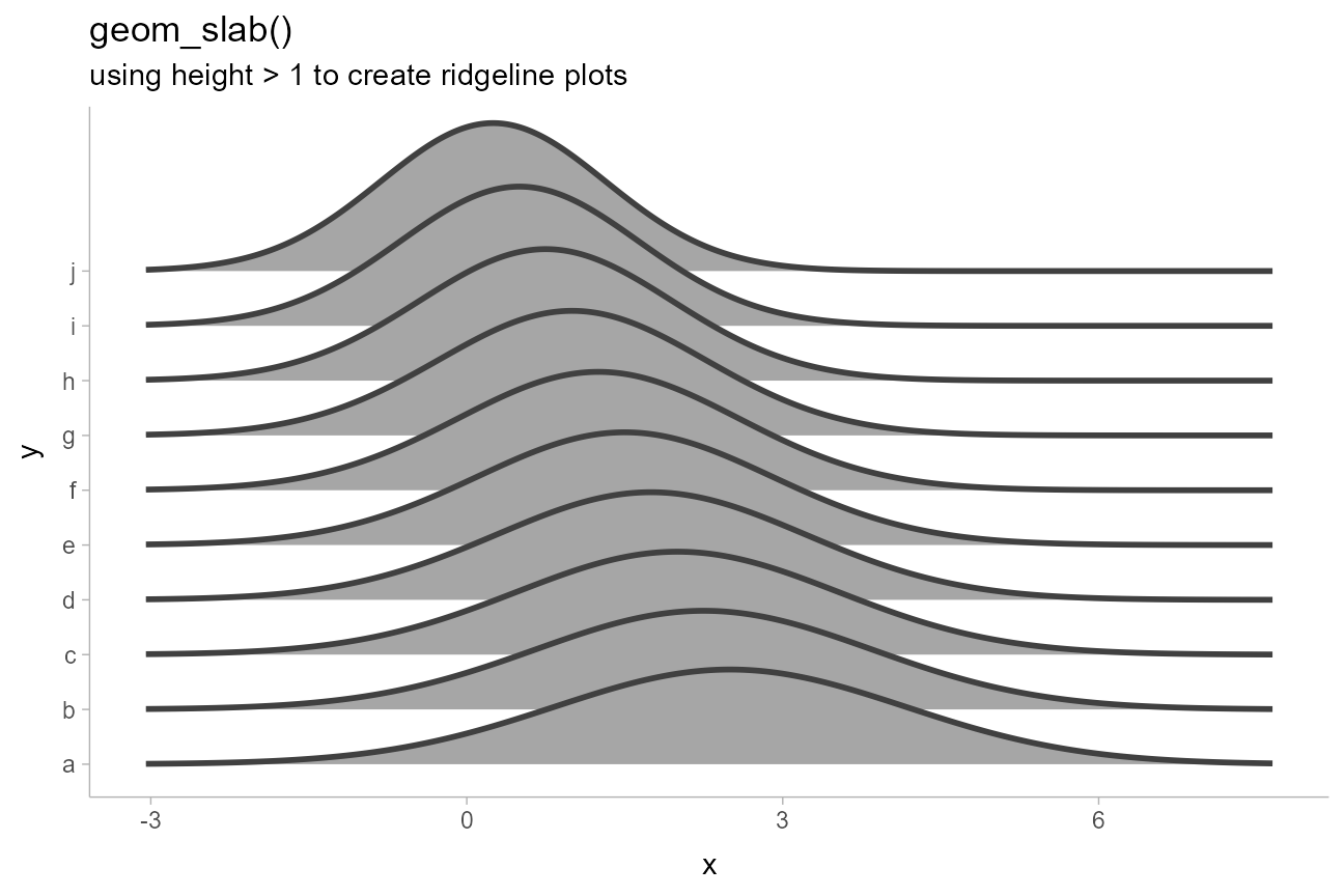
Ridgeline plots with `height > 1`

Finally, height can also be greater than 1, which can be used to create overlapping slabs, as in so-called ridgeline plots:

data.frame(
  d = dist_normal(10:1/4, 1 + 10:1/15),
  y = letters[1:10]
) %>%
  ggplot(aes(xdist = d, y = y)) +
  stat_slab(height = 3, color = "gray25") +
  labs(
    title = "geom_slab()",
    subtitle = "using height > 1 to create ridgeline plots"
  )

Matthew Kay

2024-03-04

Introduction

Setup

The `thickness` scale

Adjusting normalization within one geometry

`normalize = "all"`

`normalize = "panels"`

`normalize = "xy"`

`normalize = "groups"`

Spacing slabs with `height` and `scale`

Spacing dodged slabs

Ridgeline plots with `height > 1`

Thickness scale

Matthew Kay

2024-03-04

Introduction

Setup

The thickness scale

Adjusting normalization within one geometry

normalize = "all"

normalize = "panels"

normalize = "xy"

normalize = "groups"

Sharing thickness scales across multiple geometries

Spacing slabs with height and scale

Spacing dodged slabs

Ridgeline plots with height > 1

The `thickness` scale

`normalize = "all"`

`normalize = "panels"`

`normalize = "xy"`

`normalize = "groups"`

Sharing `thickness` scales across multiple geometries

Spacing slabs with `height` and `scale`

Ridgeline plots with `height > 1`