Dots + point + interval plot (shortcut stat)

A combination of stat_slabinterval() and geom_dotsinterval() with sensible defaults for making dots + point + interval plots. While geom_dotsinterval() is intended for use on data frames that have already been summarized using a point_interval() function, stat_dotsinterval() is intended for use directly on data frames of draws or of analytical distributions, and will perform the summarization using a point_interval() function. Geoms based on geom_dotsinterval() create dotplots that automatically determine a bin width that ensures the plot fits within the available space. They can also ensure dots do not overlap.

Usage

stat_dotsinterval(
  mapping = NULL,
  data = NULL,
  geom = "dotsinterval",
  position = "identity",
  ...,
  quantiles = NA,
  point_interval = "median_qi",
  .width = c(0.66, 0.95),
  orientation = NA,
  na.rm = FALSE,
  show.legend = c(size = FALSE),
  inherit.aes = TRUE
)

Arguments

mapping

Set of aesthetic mappings created by aes(). If specified and inherit.aes = TRUE (the default), it is combined with the default mapping at the top level of the plot. You must supply mapping if there is no plot mapping.

data

The data to be displayed in this layer. There are three options:

If NULL, the default, the data is inherited from the plot data as specified in the call to ggplot().

A data.frame, or other object, will override the plot data. All objects will be fortified to produce a data frame. See fortify() for which variables will be created.

A function will be called with a single argument, the plot data. The return value must be a data.frame, and will be used as the layer data. A function can be created from a formula (e.g. ~ head(.x, 10)).

geom

Use to override the default connection between stat_dotsinterval() and geom_dotsinterval()

position

Position adjustment, either as a string, or the result of a call to a position adjustment function. Setting this equal to "dodge" (position_dodge()) or "dodgejust" (position_dodgejust()) can be useful if you have overlapping geometries.

...

Other arguments passed to layer(). These are often aesthetics, used to set an aesthetic to a fixed value, like colour = "red" or linewidth = 3 (see Aesthetics, below). They may also be parameters to the paired geom/stat. When paired with the default geom, geom_dotsinterval(), these include:

binwidth

The bin width to use for laying out the dots. One of:

NA (the default): Dynamically select the bin width based on the size of the plot when drawn. This will pick a binwidth such that the tallest stack of dots is at most scale in height (ideally exactly scale in height, though this is not guaranteed).
A length-1 (scalar) numeric or unit object giving the exact bin width.
A length-2 (vector) numeric or unit object giving the minimum and maximum desired bin width. The bin width will be dynamically selected within these bounds.

If the value is numeric, it is assumed to be in units of data. The bin width (or its bounds) can also be specified using unit(), which may be useful if it is desired that the dots be a certain point size or a certain percentage of the width/height of the viewport. For example, unit(0.1, "npc") would make dots that are exactly 10% of the viewport size along whichever dimension the dotplot is drawn; unit(c(0, 0.1), "npc") would make dots that are at most 10% of the viewport size (while still ensuring the tallest stack is less than or equal to scale).

dotsize

The width of the dots relative to the binwidth. The default, 1.07, makes dots be just a bit wider than the bin width, which is a manually-tuned parameter that tends to work well with the default circular shape, preventing gaps between bins from appearing to be too large visually (as might arise from dots being precisely the binwidth). If it is desired to have dots be precisely the binwidth, set dotsize = 1.

stackratio

The distance between the center of the dots in the same stack relative to the dot height. The default, 1, makes dots in the same stack just touch each other.

layout

The layout method used for the dots:

"bin" (default): places dots on the off-axis at the midpoint of their bins as in the classic Wilkinson dotplot. This maintains the alignment of rows and columns in the dotplot. This layout is slightly different from the classic Wilkinson algorithm in that: (1) it nudges bins slightly to avoid overlapping bins and (2) if the input data are symmetrical it will return a symmetrical layout.
"weave": uses the same basic binning approach of "bin", but places dots in the off-axis at their actual positions (unless overlaps = "nudge", in which case overlaps may be nudged out of the way). This maintains the alignment of rows but does not align dots within columns.
"hex": uses the same basic binning approach of "bin", but alternates placing dots + binwidth/4 or - binwidth/4 in the off-axis from the bin center. This allows hexagonal packing by setting a stackratio less than 1 (something like 0.9 tends to work).
"swarm": uses the "compactswarm" layout from beeswarm::beeswarm(). Does not maintain alignment of rows or columns, but can be more compact and neat looking, especially for sample data (as opposed to quantile dotplots of theoretical distributions, which may look better with "bin", "weave", or "hex").
"bar": for discrete distributions, lays out duplicate values in rectangular bars.

overlaps

How to handle overlapping dots or bins in the "bin", "weave", and "hex" layouts (dots never overlap in the "swarm" or "bar" layouts). For the purposes of this argument, dots are only considered to be overlapping if they would be overlapping when dotsize = 1 and stackratio = 1; i.e. if you set those arguments to other values, overlaps may still occur. One of:

"keep": leave overlapping dots as they are. Dots may overlap (usually only slightly) in the "bin", "weave", and "hex" layouts.
"nudge": nudge overlapping dots out of the way. Overlaps are avoided using a constrained optimization which minimizes the squared distance of dots to their desired positions, subject to the constraint that adjacent dots do not overlap.

smooth

Smoother to apply to dot positions. One of:

A function that takes a numeric vector of dot positions and returns a smoothed version of that vector, such as smooth_bounded(), smooth_unbounded(), smooth_discrete(), or smooth_bar()`.
A string indicating what smoother to use, as the suffix to a function name starting with smooth_; e.g. "none" (the default) applies smooth_none(), which simply returns the given vector without applying smoothing.

Smoothing is most effective when the smoother is matched to the support of the distribution; e.g. using smooth_bounded(bounds = ...).

overflow

How to handle overflow of dots beyond the extent of the geom when a minimum binwidth (or an exact binwidth) is supplied. One of:

"keep": Keep the overflow, drawing dots outside the geom bounds.
"warn": Keep the overflow, but produce a warning suggesting solutions, such as setting binwidth = NA or overflow = "compress".
"compress": Compress the layout. Reduces the binwidth to the size necessary to keep the dots within bounds, then adjusts stackratio and dotsize so that the apparent dot size is the user-specified minimum binwidth times the user-specified dotsize.

If you find the default layout has dots that are too small, and you are okay with dots overlapping, consider setting overflow = "compress" and supplying an exact or minimum dot size using binwidth.

verbose

If TRUE, print out the bin width of the dotplot. Can be useful if you want to start from an automatically-selected bin width and then adjust it manually. Bin width is printed both as data units and as normalized parent coordinates or "npc"s (see unit()). Note that if you just want to scale the selected bin width to fit within a desired area, it is probably easier to use scale than to copy and scale binwidth manually, and if you just want to provide constraints on the bin width, you can pass a length-2 vector to binwidth.

interval_size_domain

A length-2 numeric vector giving the minimum and maximum of the values of the size and linewidth aesthetics that will be translated into actual sizes for intervals drawn according to interval_size_range (see the documentation for that argument.)

interval_size_range

A length-2 numeric vector. This geom scales the raw size aesthetic values when drawing interval and point sizes, as they tend to be too thick when using the default settings of scale_size_continuous(), which give sizes with a range of c(1, 6). The interval_size_domain value indicates the input domain of raw size values (typically this should be equal to the value of the range argument of the scale_size_continuous() function), and interval_size_range indicates the desired output range of the size values (the min and max of the actual sizes used to draw intervals). Most of the time it is not recommended to change the value of this argument, as it may result in strange scaling of legends; this argument is a holdover from earlier versions that did not have size aesthetics targeting the point and interval separately. If you want to adjust the size of the interval or points separately, you can also use the linewidth or point_size aesthetics; see sub-geometry-scales.

fatten_point

A multiplicative factor used to adjust the size of the point relative to the size of the thickest interval line. If you wish to specify point sizes directly, you can also use the point_size aesthetic and scale_point_size_continuous() or scale_point_size_discrete(); sizes specified with that aesthetic will not be adjusted using fatten_point.

arrow

grid::arrow() giving the arrow heads to use on the interval, or NULL for no arrows.

subguide

Sub-guide used to annotate the thickness scale. One of:

A function that takes a scale argument giving a ggplot2::Scale object and an orientation argument giving the orientation of the geometry and then returns a grid::grob that will draw the axis annotation, such as subguide_axis() (to draw a traditional axis) or subguide_none() (to draw no annotation). See subguide_axis() for a list of possibilities and examples.
A string giving the name of such a function when prefixed with "subguide"; e.g. "axis" or "none".

quantiles

Setting this to a value other than NA will produce a quantile dotplot: that is, a dotplot of quantiles from the sample or distribution (for analytical distributions, the default of NA is taken to mean 100 quantiles). The value of quantiles determines the number of quantiles to plot. See Kay et al. (2016) and Fernandes et al. (2018) for more information on quantile dotplots.

point_interval

A function from the point_interval() family (e.g., median_qi, mean_qi, mode_hdi, etc), or a string giving the name of a function from that family (e.g., "median_qi", "mean_qi", "mode_hdi", etc; if a string, the caller's environment is searched for the function, followed by the ggdist environment). This function determines the point summary (typically mean, median, or mode) and interval type (quantile interval, qi; highest-density interval, hdi; or highest-density continuous interval, hdci). Output will be converted to the appropriate x- or y-based aesthetics depending on the value of orientation. See the point_interval() family of functions for more information.

.width

The .width argument passed to point_interval: a vector of probabilities to use that determine the widths of the resulting intervals. If multiple probabilities are provided, multiple intervals per group are generated, each with a different probability interval (and value of the corresponding .width and level generated variables).

orientation

Whether this geom is drawn horizontally or vertically. One of:

NA (default): automatically detect the orientation based on how the aesthetics are assigned. Automatic detection works most of the time.
"horizontal" (or "y"): draw horizontally, using the y aesthetic to identify different groups. For each group, uses the x, xmin, xmax, and thickness aesthetics to draw points, intervals, and slabs.
"vertical" (or "x"): draw vertically, using the x aesthetic to identify different groups. For each group, uses the y, ymin, ymax, and thickness aesthetics to draw points, intervals, and slabs.

For compatibility with the base ggplot naming scheme for orientation, "x" can be used as an alias for "vertical" and "y" as an alias for "horizontal" (ggdist had an orientation parameter before base ggplot did, hence the discrepancy).

na.rm

If FALSE, the default, missing values are removed with a warning. If TRUE, missing values are silently removed.

show.legend

logical. Should this layer be included in the legends? NA, the default, includes if any aesthetics are mapped. FALSE never includes, and TRUE always includes. It can also be a named logical vector to finely select the aesthetics to display.

inherit.aes

If FALSE, overrides the default aesthetics, rather than combining with them. This is most useful for helper functions that define both data and aesthetics and shouldn't inherit behaviour from the default plot specification, e.g. borders().

Value

A ggplot2::Stat representing a dots + point + interval geometry which can be added to a ggplot() object.

Details

The dots family of stats and geoms are similar to geom_dotplot() but with a number of differences:

Dots geoms act like slabs in geom_slabinterval() and can be given x positions (or y positions when in a horizontal orientation).
Given the available space to lay out dots, the dots geoms will automatically determine how many bins to use to fit the available space.
Dots geoms use a dynamic layout algorithm that lays out dots from the center out if the input data are symmetrical, guaranteeing that symmetrical data results in a symmetrical plot. The layout algorithm also prevents dots from overlapping each other.
The shape of the dots in these geoms can be changed using the slab_shape aesthetic (when using the dotsinterval family) or the shape or slab_shape aesthetic (when using the dots family)

Stats and geoms in this family include:

geom_dots(): dotplots on raw data. Ensures the dotplot fits within available space by reducing the size of the dots automatically (may result in very small dots).
geom_swarm() and geom_weave(): dotplots on raw data with defaults intended to create "beeswarm" plots. Used side = "both" by default, and sets the default dot size to the same size as geom_point() (binwidth = unit(1.5, "mm")), allowing dots to overlap instead of getting very small.
stat_dots(): dotplots on raw data, distributional objects, and posterior::rvar()s
geom_dotsinterval(): dotplot + interval plots on raw data with already-calculated intervals (rarely useful directly).
stat_dotsinterval(): dotplot + interval plots on raw data, distributional objects, and posterior::rvar()s (will calculate intervals for you).
geom_blur_dots(): blurry dotplots that allow the standard deviation of a blur applied to each dot to be specified using the sd aesthetic.
stat_mcse_dots(): blurry dotplots of quantiles using the Monte Carlo Standard Error of each quantile.

stat_dots() and stat_dotsinterval(), when used with the quantiles argument, are particularly useful for constructing quantile dotplots, which can be an effective way to communicate uncertainty using a frequency framing that may be easier for laypeople to understand (Kay et al. 2016, Fernandes et al. 2018).

To visualize sample data, such as a data distribution, samples from a bootstrap distribution, or a Bayesian posterior, you can supply samples to the x or y aesthetic.

To visualize analytical distributions, you can use the xdist or ydist aesthetic. For historical reasons, you can also use dist to specify the distribution, though this is not recommended as it does not work as well with orientation detection. These aesthetics can be used as follows:

xdist, ydist, and dist can be any distribution object from the distributional package (dist_normal(), dist_beta(), etc) or can be a posterior::rvar() object. Since these functions are vectorized, other columns can be passed directly to them in an aes() specification; e.g. aes(dist = dist_normal(mu, sigma)) will work if mu and sigma are columns in the input data frame.
dist can be a character vector giving the distribution name. Then the arg1, ... arg9 aesthetics (or args as a list column) specify distribution arguments. Distribution names should correspond to R functions that have "p", "q", and "d" functions; e.g. "norm" is a valid distribution name because R defines the pnorm(), qnorm(), and dnorm() functions for Normal distributions.

See the parse_dist() function for a useful way to generate dist and args values from human-readable distribution specs (like "normal(0,1)"). Such specs are also produced by other packages (like the brms::get_prior function in brms); thus, parse_dist() combined with the stats described here can help you visualize the output of those functions.

Computed Variables

The following variables are computed by this stat and made available for use in aesthetic specifications (aes()) using the after_stat() function or the after_stat argument of stage():

x or y: For slabs, the input values to the slab function. For intervals, the point summary from the interval function. Whether it is x or y depends on orientation
xmin or ymin: For intervals, the lower end of the interval from the interval function.
xmax or ymax: For intervals, the upper end of the interval from the interval function.
.width: For intervals, the interval width as a numeric value in [0, 1]. For slabs, the width of the smallest interval containing that value of the slab.
level: For intervals, the interval width as an ordered factor. For slabs, the level of the smallest interval containing that value of the slab.
pdf: For slabs, the probability density function (PDF). If options("ggdist.experimental.slab_data_in_intervals") is TRUE: For intervals, the PDF at the point summary; intervals also have pdf_min and pdf_max for the PDF at the lower and upper ends of the interval.
cdf: For slabs, the cumulative distribution function. If options("ggdist.experimental.slab_data_in_intervals") is TRUE: For intervals, the CDF at the point summary; intervals also have cdf_min and cdf_max for the CDF at the lower and upper ends of the interval.
n: For slabs, the number of data points summarized into that slab. If the slab was created from an analytical distribution via the xdist, ydist, or dist aesthetic, n will be Inf.
f: (deprecated) For slabs, the output values from the slab function (such as the PDF, CDF, or CCDF), determined by slab_type. Instead of using slab_type to change f and then mapping f onto an aesthetic, it is now recommended to simply map the corresponding computed variable (e.g. pdf, cdf, or 1 - cdf) directly onto the desired aesthetic.

Aesthetics

The dots+interval stats and geoms have a wide variety of aesthetics that control the appearance of their three sub-geometries: the dots (aka the slab), the point, and the interval.

These stats support the following aesthetics:

x: x position of the geometry (when orientation = "vertical"); or sample data to be summarized (when orientation = "horizontal" with sample data).
y: y position of the geometry (when orientation = "horizontal"); or sample data to be summarized (when orientation = "vertical" with sample data).
weight: When using samples (i.e. the x and y aesthetics, not xdist or ydist), optional weights to be applied to each draw.
xdist: When using analytical distributions, distribution to map on the x axis: a distributional object (e.g. dist_normal()) or a posterior::rvar() object.
ydist: When using analytical distributions, distribution to map on the y axis: a distributional object (e.g. dist_normal()) or a posterior::rvar() object.
dist: When using analytical distributions, a name of a distribution (e.g. "norm"), a distributional object (e.g. dist_normal()), or a posterior::rvar() object. See Details.
args: Distribution arguments (args or arg1, ... arg9). See Details.

In addition, in their default configuration (paired with geom_dotsinterval()) the following aesthetics are supported by the underlying geom:

Dots-specific (aka Slab-specific) aesthetics

family: The font family used to draw the dots.
order: The order in which data points are stacked within bins. Can be used to create the effect of "stacked" dots by ordering dots according to a discrete variable. If omitted (NULL), the value of the data points themselves are used to determine stacking order. Only applies when layout is "bin" or "hex", as the other layout methods fully determine both x and y positions.
side: Which side to place the slab on. "topright", "top", and "right" are synonyms which cause the slab to be drawn on the top or the right depending on if orientation is "horizontal" or "vertical". "bottomleft", "bottom", and "left" are synonyms which cause the slab to be drawn on the bottom or the left depending on if orientation is "horizontal" or "vertical". "topleft" causes the slab to be drawn on the top or the left, and "bottomright" causes the slab to be drawn on the bottom or the right. "both" draws the slab mirrored on both sides (as in a violin plot).
scale: What proportion of the region allocated to this geom to use to draw the slab. If scale = 1, slabs that use the maximum range will just touch each other. Default is 0.9 to leave some space between adjacent slabs. For a comprehensive discussion and examples of slab scaling and normalization, see the thickness scale article.
justification: Justification of the interval relative to the slab, where 0 indicates bottom/left justification and 1 indicates top/right justification (depending on orientation). If justification is NULL (the default), then it is set automatically based on the value of side: when side is "top"/"right" justification is set to 0, when side is "bottom"/"left" justification is set to 1, and when side is "both" justification is set to 0.5.
datatype: When using composite geoms directly without a stat (e.g. geom_slabinterval()), datatype is used to indicate which part of the geom a row in the data targets: rows with datatype = "slab" target the slab portion of the geometry and rows with datatype = "interval" target the interval portion of the geometry. This is set automatically when using ggdist stats.

Interval-specific aesthetics

xmin: Left end of the interval sub-geometry (if orientation = "horizontal").
xmax: Right end of the interval sub-geometry (if orientation = "horizontal").
ymin: Lower end of the interval sub-geometry (if orientation = "vertical").
ymax: Upper end of the interval sub-geometry (if orientation = "vertical").

Point-specific aesthetics

shape: Shape type used to draw the point sub-geometry.

Color aesthetics

colour: (or color) The color of the interval and point sub-geometries. Use the slab_color, interval_color, or point_color aesthetics (below) to set sub-geometry colors separately.
fill: The fill color of the slab and point sub-geometries. Use the slab_fill or point_fill aesthetics (below) to set sub-geometry colors separately.
alpha: The opacity of the slab, interval, and point sub-geometries. Use the slab_alpha, interval_alpha, or point_alpha aesthetics (below) to set sub-geometry colors separately.
colour_ramp: (or color_ramp) A secondary scale that modifies the color scale to "ramp" to another color. See scale_colour_ramp() for examples.
fill_ramp: A secondary scale that modifies the fill scale to "ramp" to another color. See scale_fill_ramp() for examples.

Line aesthetics

linewidth: Width of the line used to draw the interval (except with geom_slab(): then it is the width of the slab). With composite geometries including an interval and slab, use slab_linewidth to set the line width of the slab (see below). For interval, raw linewidth values are transformed according to the interval_size_domain and interval_size_range parameters of the geom (see above).
size: Determines the size of the point. If linewidth is not provided, size will also determines the width of the line used to draw the interval (this allows line width and point size to be modified together by setting only size and not linewidth). Raw size values are transformed according to the interval_size_domain, interval_size_range, and fatten_point parameters of the geom (see above). Use the point_size aesthetic (below) to set sub-geometry size directly without applying the effects of interval_size_domain, interval_size_range, and fatten_point.
stroke: Width of the outline around the point sub-geometry.
linetype: Type of line (e.g., "solid", "dashed", etc) used to draw the interval and the outline of the slab (if it is visible). Use the slab_linetype or interval_linetype aesthetics (below) to set sub-geometry line types separately.

Slab-specific color and line override aesthetics

slab_fill: Override for fill: the fill color of the slab.
slab_colour: (or slab_color) Override for colour/color: the outline color of the slab.
slab_alpha: Override for alpha: the opacity of the slab.
slab_linewidth: Override for linwidth: the width of the outline of the slab.
slab_linetype: Override for linetype: the line type of the outline of the slab.
slab_shape: Override for shape: the shape of the dots used to draw the dotplot slab.

Interval-specific color and line override aesthetics

interval_colour: (or interval_color) Override for colour/color: the color of the interval.
interval_alpha: Override for alpha: the opacity of the interval.
interval_linetype: Override for linetype: the line type of the interval.

Point-specific color and line override aesthetics

point_fill: Override for fill: the fill color of the point.
point_colour: (or point_color) Override for colour/color: the outline color of the point.
point_alpha: Override for alpha: the opacity of the point.
point_size: Override for size: the size of the point.

Deprecated aesthetics

slab_size: Use slab_linewidth.
interval_size: Use interval_linewidth.

Other aesthetics (these work as in standard geoms)

width
height
group

See examples of some of these aesthetics in action in vignette("dotsinterval"). Learn more about the sub-geom override aesthetics (like interval_color) in the scales documentation. Learn more about basic ggplot aesthetics in vignette("ggplot2-specs").

References

Kay, M., Kola, T., Hullman, J. R., & Munson, S. A. (2016). When (ish) is My Bus? User-centered Visualizations of Uncertainty in Everyday, Mobile Predictive Systems. Conference on Human Factors in Computing Systems - CHI '16, 5092--5103. doi:10.1145/2858036.2858558 .

Fernandes, M., Walls, L., Munson, S., Hullman, J., & Kay, M. (2018). Uncertainty Displays Using Quantile Dotplots or CDFs Improve Transit Decision-Making. Conference on Human Factors in Computing Systems - CHI '18. doi:10.1145/3173574.3173718 .

Examples

library(dplyr)
library(ggplot2)
library(distributional)

theme_set(theme_ggdist())

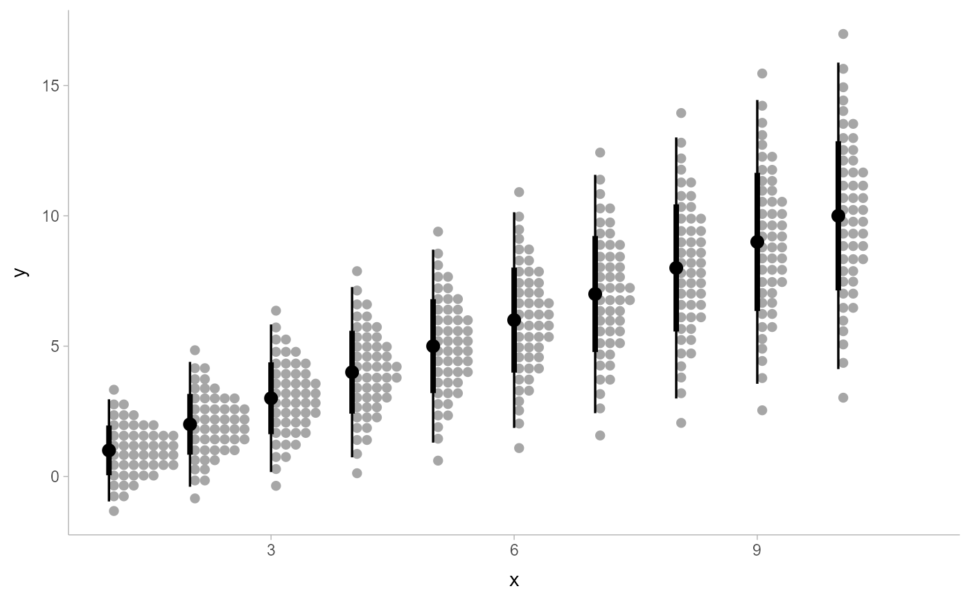
# ON SAMPLE DATA
set.seed(12345)
tibble(
  x = rep(1:10, 100),
  y = rnorm(1000, x)
) %>%
  ggplot(aes(x = x, y = y)) +
  stat_dotsinterval()


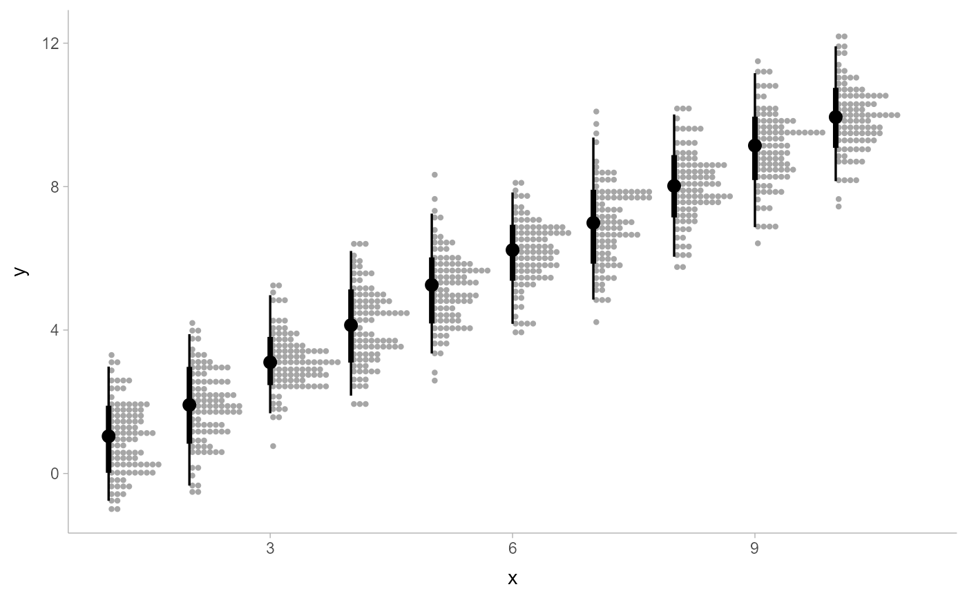# ON ANALYTICAL DISTRIBUTIONS
# Vectorized distribution types, like distributional::dist_normal()
# and posterior::rvar(), can be used with the `xdist` / `ydist` aesthetics
tibble(
  x = 1:10,
  sd = seq(1, 3, length.out = 10)
) %>%
  ggplot(aes(x = x, ydist = dist_normal(x, sd))) +
  stat_dotsinterval(quantiles = 50)