Scaled and shifted Student's t distribution

Density, distribution function, quantile function and random generation for the scaled and shifted Student's t distribution, parameterized by degrees of freedom (df), location (mu), and scale (sigma).

Usage

dstudent_t(x, df, mu = 0, sigma = 1, log = FALSE)

pstudent_t(q, df, mu = 0, sigma = 1, lower.tail = TRUE, log.p = FALSE)

qstudent_t(p, df, mu = 0, sigma = 1, lower.tail = TRUE, log.p = FALSE)

rstudent_t(n, df, mu = 0, sigma = 1)

Arguments

x, q

vector of quantiles.

df

degrees of freedom (\(> 0\), maybe non-integer). df = Inf is allowed.

mu

Location parameter (median)

sigma

Scale parameter

log, log.p

logical; if TRUE, probabilities p are given as log(p).

lower.tail

logical; if TRUE (default), probabilities are \(P[X \le x]\), otherwise, \(P[X > x]\).

p

vector of probabilities.

n

number of observations. If length(n) > 1, the length is taken to be the number required.

Value

• dstudent_t gives the density

• pstudent_t gives the cumulative distribution function (CDF)

• qstudent_t gives the quantile function (inverse CDF)

• rstudent_t generates random draws.

The length of the result is determined by n for rstudent_t, and is the maximum of the lengths of the numerical arguments for the other functions.

The numerical arguments other than n are recycled to the length of the result. Only the first elements of the logical arguments are used.

See also

parse_dist() and parsing distribution specs and the stat_slabinterval() family of stats for visualizing them.

Examples

library(dplyr)
library(ggplot2)

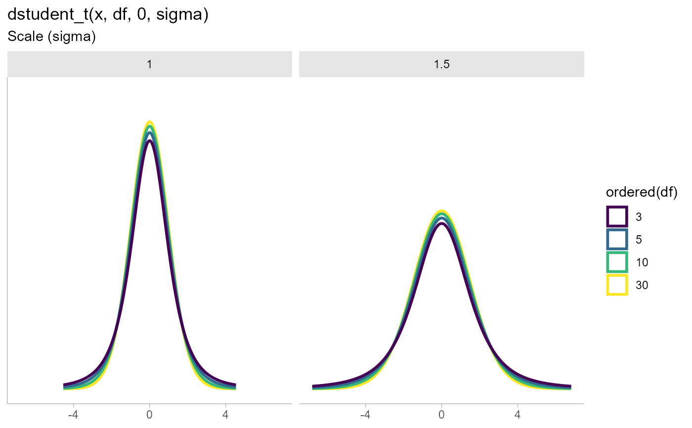
expand.grid(
  df = c(3,5,10,30),
  scale = c(1,1.5)
) %>%
  ggplot(aes(y = 0, dist = "student_t", arg1 = df, arg2 = 0, arg3 = scale, color = ordered(df))) +
  stat_slab(p_limits = c(.01, .99), fill = NA) +
  scale_y_continuous(breaks = NULL) +
  facet_grid( ~ scale) +
  labs(
    title = "dstudent_t(x, df, 0, sigma)",
    subtitle = "Scale (sigma)",
    y = NULL,
    x = NULL
  ) +
  theme_ggdist() +
  theme(axis.title = element_text(hjust = 0))