Turn spec for LKJ distribution into spec for marginal LKJ distribution

Turns specs for an LKJ correlation matrix distribution as returned by parse_dist() into specs for the marginal distribution of a single cell in an LKJ-distributed correlation matrix (i.e., lkjcorr_marginal()). Useful for visualizing prior correlations from LKJ distributions.

Usage

marginalize_lkjcorr(
  data,
  K,
  predicate = NULL,
  dist = ".dist",
  args = ".args",
  dist_obj = ".dist_obj"
)

Arguments

data

A data frame containing a column with distribution names (".dist" by default) and a list column of distribution arguments (".args" by default), such as output by parse_dist().

K

Dimension of the correlation matrix. Must be greater than or equal to 2.

predicate

a bare expression for selecting the rows of data to modify. This is useful if data contains more than one row with an LKJ prior in it and you only want to modify some of the distributions; if this is the case, give row a predicate expression that evaluates to TRUE on the rows you want to modify. If NULL (the default), all lkjcorr distributions in data are modified.

dist

The name of the column containing distribution names. See parse_dist().

args

The name of the column containing distribution arguments. See parse_dist().

dist_obj

The name of the column to contain a distributional object representing the distribution. See parse_dist().

Value

A data frame of the same size and column names as the input, with the dist, and args, and dist_obj columns modified on rows where dist == "lkjcorr" such that they represent a marginal LKJ correlation distribution with name lkjcorr_marginal and args having K equal to the input value of K.

Details

The LKJ(eta) prior on a correlation matrix induces a marginal prior on each correlation in the matrix that depends on both the value of eta and K, the dimension of the \(K \times K\) correlation matrix. Thus to visualize the marginal prior on the correlations, it is necessary to specify the value of K, which depends on what your model specification looks like.

Given a data frame representing parsed distribution specifications (such as returned by parse_dist()), this function updates any rows with .dist == "lkjcorr" so that the first argument to the distribution (stored in .args) is equal to the specified dimension of the correlation matrix (K), changes the distribution name in .dist to "lkjcorr_marginal", and assigns a distributional object representing this distribution to .dist_obj. This allows the distribution to be easily visualized using the stat_slabinterval() family of ggplot2 stats.

See also

parse_dist(), lkjcorr_marginal()

Examples

library(dplyr)
library(ggplot2)

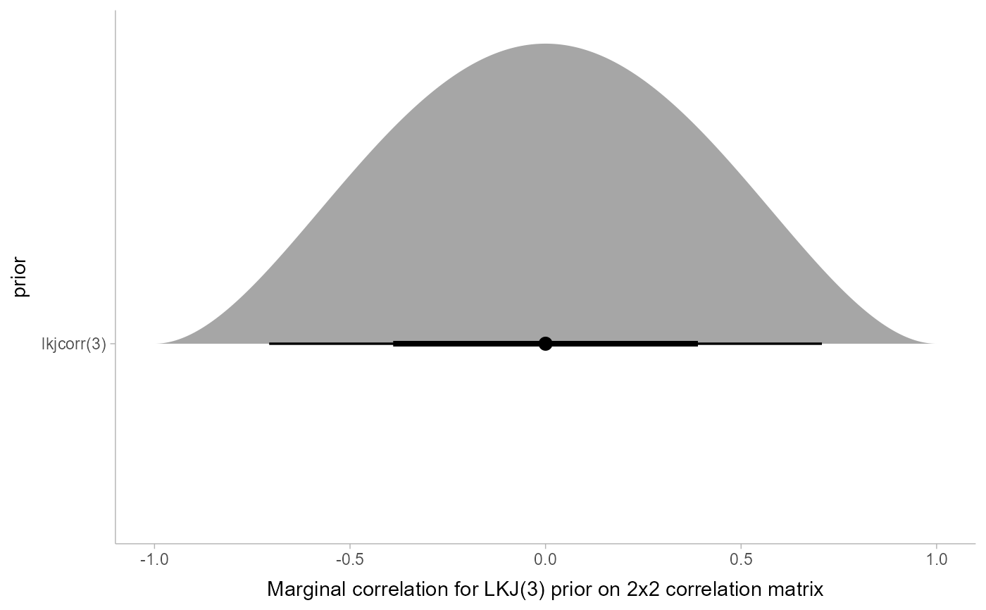
# Say we have an LKJ(3) prior on a 2x2 correlation matrix. We can visualize
# its marginal distribution as follows...
data.frame(prior = "lkjcorr(3)") %>%
  parse_dist(prior) %>%
  marginalize_lkjcorr(K = 2) %>%
  ggplot(aes(y = prior, xdist = .dist_obj)) +
  stat_halfeye() +
  xlim(-1, 1) +
  xlab("Marginal correlation for LKJ(3) prior on 2x2 correlation matrix")


# Say our prior list has multiple LKJ priors on correlation matrices
# of different sizes, we can supply a predicate expression to select
# only those rows we want to modify
data.frame(coef = c("a", "b"), prior = "lkjcorr(3)") %>%
  parse_dist(prior) %>%
  marginalize_lkjcorr(K = 2, coef == "a") %>%
  marginalize_lkjcorr(K = 4, coef == "b")
#>   coef      prior            .dist .args              .dist_obj
#> 1    a lkjcorr(3) lkjcorr_marginal  2, 3 lkjcorr_marginal(2, 3)
#> 2    b lkjcorr(3) lkjcorr_marginal  4, 3 lkjcorr_marginal(4, 3)