Nicely-spaced sets of interval widths

Create nicely-spaced sets of nested interval widths for use with (e.g.) the .width parameter of point_interval(), stat_slabinterval(), or stat_lineribbon():

interval_widths(n) creates a sequence of n interval widths $p_1 \ldots p_n$, where $0 < p_i \le \textrm{max} < 1$, corresponding to the masses of nested intervals that are evenly-spaced on a reference distribution (by default a Normal distribution). This generalizes the idea behind the default ~66% and 95% intervals in stat_slabinterval() and 50%, 80%, and 95% intervals in stat_lineribbon(): when applied to a Normal distribution, those intervals are roughly evenly-spaced and allow one to see deviations from the reference distribution (such as excess kurtosis) when the resulting intervals are not evenly spaced.
pretty_widths(n) is a variant of interval_widths() with defaults for max and precision that make the resulting intervals more human-readable, for labeling purposes.

Intervals should be evenly-spaced on any symmetric reference distribution when applied to data from distributions with the same shape. If dist is not symmetric, intervals may only be approximately evenly-spaced above the median.

Usage

interval_widths(n, dist = dist_normal(), max = 1 - 0.1/n, precision = NULL)

pretty_widths(
  n,
  dist = dist_normal(),
  max = if (n <= 4) 0.95 else 1 - 0.1/n,
  precision = if (n <= 4) 0.05 else 0.01
)

Arguments

n: <numeric> in $[0, \infty)$: Number of intervals to generate.
dist: <distribution>: Reference distribution.
max: <numeric> in $(0, 1)$: Maximum interval width.
precision: <numeric | NULL>: If not NULL, a value in $(0, 1)$ giving the precision to round resulting widths to. In order to guarantee n unique intervals are returned, widths will only be rounded if the result does not create duplicate values.

Value

A length-n numeric vector of interval widths (masses) between 0 and 1 (exclusive) in increasing order.

Details

Given the cumulative distribution function $F_\textrm{dist}(q)$ and the quantile function $F^{-1}_\textrm{dist}(p)$ of dist, the following is a sequence of $n + 1$ evenly-spaced quantiles of dist that could represent upper limits of nested intervals, where $q_i = q_0 + i\frac{q_n - q_0}{n}$:

$$\begin{array}{rcl} q_0, \ldots, q_n &=& F^{-1}_\textrm{dist}(0.5), \ldots, F^{-1}_\textrm{dist}(0.5 + \frac{\textrm{max}}{2}) \end{array}$$

interval_widths(n) returns the n interval widths corresponding to the upper interval limits $q_1, \ldots, q_n$:

$$ 2\cdot\left[F_\textrm{dist}(q_1) - 0.5\right], \ldots, 2\cdot\left[F_\textrm{dist}(q_n) - 0.5\right] $$

Examples

library(ggplot2)
library(distributional)

interval_widths(1)   # 0.9
#> [1] 0.9
# this is roughly +/- 1 SD and +/- 2 SD
interval_widths(2)   # 0.672..., 0.95
#> [1] 0.672905 0.950000
interval_widths(3)   # 0.521..., 0.844..., 0.966...
#> [1] 0.5218917 0.8440126 0.9666667

# "pretty" widths may be useful for legends with a small number of widths
pretty_widths(1)     # 0.95
#> [1] 0.95
pretty_widths(2)     # 0.65, 0.95
#> [1] 0.65 0.95
pretty_widths(3)     # 0.50, 0.80, 0.95
#> [1] 0.50 0.80 0.95

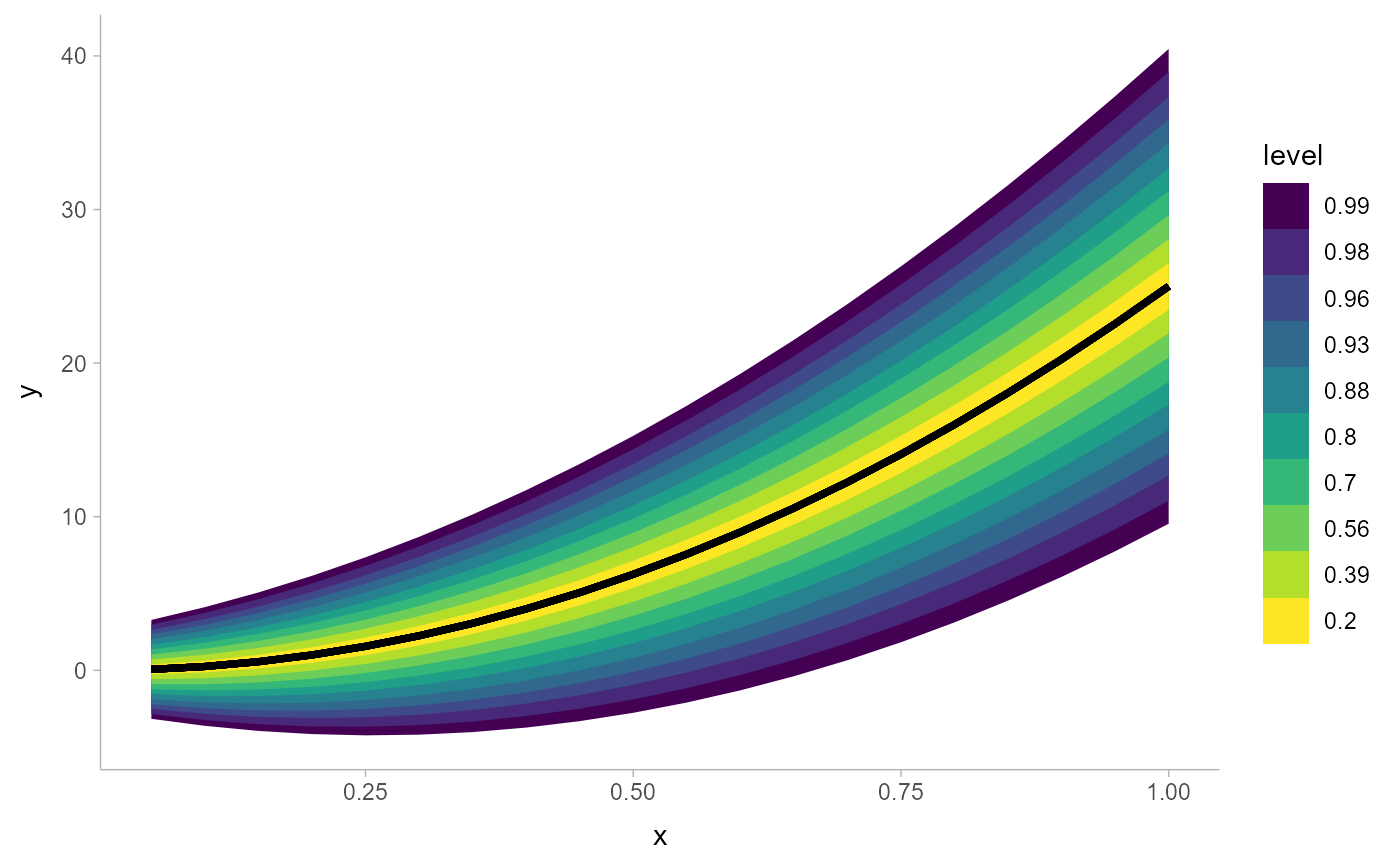
# larger numbers of intervals can be useful for plots
ggplot(data.frame(x = 1:20/20)) +
  aes(x, ydist = dist_normal((x * 5)^2, 1 + x * 5)) +
  stat_lineribbon(.width = pretty_widths(10))


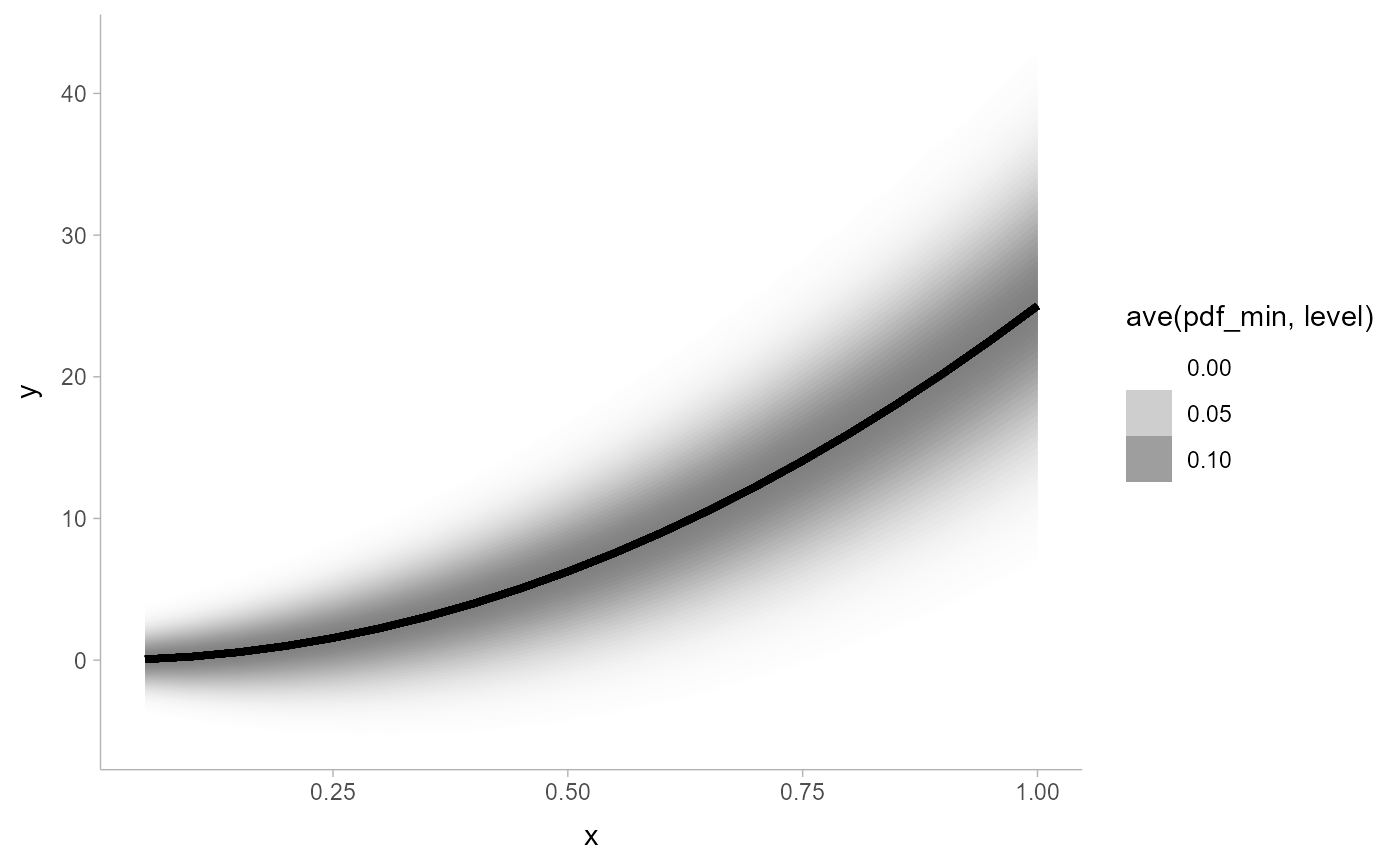
# large numbers of intervals can be used to create gradients -- particularly
# useful if you shade ribbons according to density (not interval width)
# (this is currently experimental)
withr::with_options(list(ggdist.experimental.slab_data_in_intervals = TRUE), print(
  ggplot(data.frame(x = 1:20/20)) +
    aes(x, ydist = dist_normal((x * 5)^2, 1 + x * 5)) +
    stat_lineribbon(
      aes(fill_ramp = after_stat(ave(pdf_min, level))),
      .width = interval_widths(40),
      fill = "gray50"
    ) +
    theme_ggdist()
))

Usage

Arguments

Value

Details

See also

Examples