Bins the provided data values using one of several dotplot algorithms.
Arguments
- x
<numeric> x values.
- y
<numeric> y values (same length as
x).- binwidth
<scalar numeric> Bin width.
- heightratio
<scalar numeric> Ratio of bin width to dot height
- stackratio
<scalar numeric> Ratio of dot height to vertical distance between dot centers
- layout
<string> The layout method used for the dots. One of:
"bin"(default): places dots on the off-axis at the midpoint of their bins as in the classic Wilkinson dotplot. This maintains the alignment of rows and columns in the dotplot. This layout is slightly different from the classic Wilkinson algorithm in that: (1) it nudges bins slightly to avoid overlapping bins and (2) if the input data are symmetrical it will return a symmetrical layout."weave": uses the same basic binning approach of"bin", but places dots in the off-axis at their actual positions (unlessoverlaps = "nudge", in which case overlaps may be nudged out of the way). This maintains the alignment of rows but does not align dots within columns."hex": uses the same basic binning approach of"bin", but alternates placing dots+ binwidth/4or- binwidth/4in the off-axis from the bin center. This allows hexagonal packing by setting astackratioless than 1 (something like0.9tends to work)."swarm": uses a version of the"compactswarm"layout frombeeswarm::beeswarm()(with minor modifications to improve visual symmetry whenside = "both"). Does not maintain alignment of rows or columns, but can be more compact and neat-looking, especially for sample data (as opposed to quantile dotplots of theoretical distributions, which may look better with"bin","weave", or"hex")."bar": for discrete distributions, lays out duplicate values in rectangular bars.
- side
Which side to place the slab on.
"topright","top", and"right"are synonyms which cause the slab to be drawn on the top or the right depending on iforientationis"horizontal"or"vertical"."bottomleft","bottom", and"left"are synonyms which cause the slab to be drawn on the bottom or the left depending on iforientationis"horizontal"or"vertical"."topleft"causes the slab to be drawn on the top or the left, and"bottomright"causes the slab to be drawn on the bottom or the right."both"draws the slab mirrored on both sides (as in a violin plot).- orientation
<string> Whether the dots are laid out horizontally or vertically. Follows the naming scheme of
geom_slabinterval():"horizontal"assumes the data values for the dotplot are in thexvariable and that dots will be stacked up in theydirection."vertical"assumes the data values for the dotplot are in theyvariable and that dots will be stacked up in thexdirection.
For compatibility with the base ggplot naming scheme for
orientation,"x"can be used as an alias for"vertical"and"y"as an alias for"horizontal".- overlaps
<string> How to handle overlapping dots or bins in the
"bin","weave", and"hex"layouts (dots never overlap in the"swarm"or"bar"layouts). For the purposes of this argument, dots are only considered to be overlapping if they would be overlapping whendotsize = 1andstackratio = 1; i.e. if you set those arguments to other values, overlaps may still occur. One of:"keep": leave overlapping dots as they are. Dots may overlap (usually only slightly) in the"bin","weave", and"hex"layouts."nudge": nudge overlapping dots out of the way. Overlaps are avoided using a constrained optimization which minimizes the squared distance of dots to their desired positions, subject to the constraint that adjacent dots do not overlap.
Value
A data.frame with three columns:
x: the x position of each doty: the y position of each dotbin: a unique number associated with each bin (supplied but not used whenlayout = "swarm")
See also
find_dotplot_binwidth() for an algorithm that finds good bin widths
to use with this function; geom_dotsinterval() for geometries that use
these algorithms to create dotplots.
Examples
library(dplyr)
#>
#> Attaching package: 'dplyr'
#> The following objects are masked from 'package:stats':
#>
#> filter, lag
#> The following objects are masked from 'package:base':
#>
#> intersect, setdiff, setequal, union
library(ggplot2)
x = qnorm(ppoints(20))
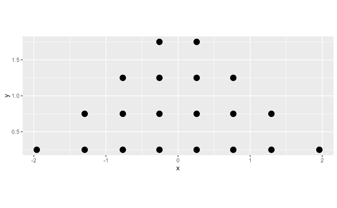
bin_df = bin_dots(x = x, y = 0, binwidth = 0.5, heightratio = 1)
bin_df
#> x y bin
#> 1 -1.9599640 0.25 1
#> 2 -1.2949404 0.25 2
#> 3 -1.2949404 0.75 2
#> 4 -0.7661747 0.25 3
#> 5 -0.7661747 0.75 3
#> 6 -0.7661747 1.25 3
#> 7 -0.2582345 0.25 4
#> 8 -0.2582345 0.75 4
#> 9 -0.2582345 1.25 4
#> 10 -0.2582345 1.75 4
#> 11 0.2582345 0.25 5
#> 12 0.2582345 0.75 5
#> 13 0.2582345 1.25 5
#> 14 0.2582345 1.75 5
#> 15 0.7661747 0.25 6
#> 16 0.7661747 0.75 6
#> 17 0.7661747 1.25 6
#> 18 1.2949404 0.25 7
#> 19 1.2949404 0.75 7
#> 20 1.9599640 0.25 8
# we can manually plot the binning above, though this is only recommended
# if you are using find_dotplot_binwidth() and bin_dots() to build your own
# grob. For practical use it is much easier to use geom_dots(), which will
# automatically select good bin widths for you (and which uses
# find_dotplot_binwidth() and bin_dots() internally)
bin_df %>%
ggplot(aes(x = x, y = y)) +
geom_point(size = 4) +
coord_fixed()