Add rvars for the linear predictor, posterior expectation, posterior predictive, or residuals of a model to a data frame

Given a data frame and a model, adds rvars of draws from the linear/link-level predictor, the expectation of the posterior predictive, or the posterior predictive to the data frame.

add_epred_rvars(
  newdata,
  object,
  ...,
  value = ".epred",
  ndraws = NULL,
  seed = NULL,
  re_formula = NULL,
  dpar = NULL,
  columns_to = NULL
)

epred_rvars(
  object,
  newdata,
  ...,
  value = ".epred",
  ndraws = NULL,
  seed = NULL,
  re_formula = NULL,
  dpar = NULL,
  columns_to = NULL
)

# S3 method for default
epred_rvars(
  object,
  newdata,
  ...,
  value = ".epred",
  seed = NULL,
  dpar = NULL,
  columns_to = NULL
)

# S3 method for stanreg
epred_rvars(
  object,
  newdata,
  ...,
  value = ".epred",
  ndraws = NULL,
  seed = NULL,
  re_formula = NULL,
  dpar = NULL,
  columns_to = NULL
)

# S3 method for brmsfit
epred_rvars(
  object,
  newdata,
  ...,
  value = ".epred",
  ndraws = NULL,
  seed = NULL,
  re_formula = NULL,
  dpar = NULL,
  columns_to = NULL
)

add_linpred_rvars(
  newdata,
  object,
  ...,
  value = ".linpred",
  ndraws = NULL,
  seed = NULL,
  re_formula = NULL,
  dpar = NULL,
  columns_to = NULL
)

linpred_rvars(
  object,
  newdata,
  ...,
  value = ".linpred",
  ndraws = NULL,
  seed = NULL,
  re_formula = NULL,
  dpar = NULL,
  columns_to = NULL
)

# S3 method for default
linpred_rvars(
  object,
  newdata,
  ...,
  value = ".linpred",
  seed = NULL,
  dpar = NULL,
  columns_to = NULL
)

# S3 method for stanreg
linpred_rvars(
  object,
  newdata,
  ...,
  value = ".linpred",
  ndraws = NULL,
  seed = NULL,
  re_formula = NULL,
  dpar = NULL,
  columns_to = NULL
)

# S3 method for brmsfit
linpred_rvars(
  object,
  newdata,
  ...,
  value = ".linpred",
  ndraws = NULL,
  seed = NULL,
  re_formula = NULL,
  dpar = NULL,
  columns_to = NULL
)

add_predicted_rvars(
  newdata,
  object,
  ...,
  value = ".prediction",
  ndraws = NULL,
  seed = NULL,
  re_formula = NULL,
  columns_to = NULL
)

predicted_rvars(
  object,
  newdata,
  ...,
  value = ".prediction",
  ndraws = NULL,
  seed = NULL,
  re_formula = NULL,
  columns_to = NULL
)

# S3 method for default
predicted_rvars(
  object,
  newdata,
  ...,
  value = ".prediction",
  seed = NULL,
  columns_to = NULL
)

# S3 method for stanreg
predicted_rvars(
  object,
  newdata,
  ...,
  value = ".prediction",
  ndraws = NULL,
  seed = NULL,
  re_formula = NULL,
  columns_to = NULL
)

# S3 method for brmsfit
predicted_rvars(
  object,
  newdata,
  ...,
  value = ".prediction",
  ndraws = NULL,
  seed = NULL,
  re_formula = NULL,
  columns_to = NULL
)

Arguments

newdata

Data frame to generate predictions from.

object

A supported Bayesian model fit that can provide fits and predictions. Supported models are listed in the second section of tidybayes-models: Models Supporting Prediction. While other functions in this package (like spread_rvars()) support a wider range of models, to work with add_epred_rvars(), add_predicted_rvars(), etc. a model must provide an interface for generating predictions, thus more generic Bayesian modeling interfaces like runjags and rstan are not directly supported for these functions (only wrappers around those languages that provide predictions, like rstanarm and brm, are supported here).

...

Additional arguments passed to the underlying prediction method for the type of model given.

value

The name of the output column:

for [add_]epred_rvars(), defaults to ".epred".
for [add_]predicted_rvars(), defaults to ".prediction".
for [add_]linpred_rvars(), defaults to ".linpred".

ndraws

The number of draws to return, or NULL to return all draws.

seed

A seed to use when subsampling draws (i.e. when ndraws is not NULL).

re_formula

formula containing group-level effects to be considered in the prediction. If NULL (default), include all group-level effects; if NA, include no group-level effects. Some model types (such as brms::brmsfit and rstanarm::stanreg-objects) allow marginalizing over grouping factors by specifying new levels of a factor in newdata. In the case of brms::brm(), you must also pass allow_new_levels = TRUE here to include new levels (see brms::posterior_predict()).

dpar

For add_epred_rvars() and add_linpred_rvars(): Should distributional regression parameters be included in the output? Valid only for models that support distributional regression parameters, such as submodels for variance parameters (as in brms::brm()). If TRUE, distributional regression parameters are included in the output as additional columns named after each parameter (alternative names can be provided using a list or named vector, e.g. c(sigma.hat = "sigma") would output the "sigma" parameter from a model as a column named "sigma.hat"). If NULL or FALSE (the default), distributional regression parameters are not included.

columns_to

For some models, such as ordinal, multinomial, and multivariate models (notably, brms::brm() models but not rstanarm::stan_polr() models), the column of predictions in the resulting data frame may include nested columns. For example, for ordinal/multinomial models, these columns correspond to different categories of the response variable. It may be more convenient to turn these nested columns into rows in the output; if this is desired, set columns_to to a string representing the name of a column you would like the column names to be placed in. In this case, a .row column will also be added to the result indicating which rows of the output correspond to the same row in newdata. See vignette("tidy-posterior") for examples of dealing with output ordinal models.

Value

A data frame (actually, a tibble) equal to the input newdata with additional columns added containing rvars representing the requested predictions or fits.

Details

Consider a model like:

$$\begin{array}{rcl} y &\sim& \textrm{SomeDist}(\theta_1, \theta_2)\\ f_1(\theta_1) &=& \alpha_1 + \beta_1 x\\ f_2(\theta_2) &=& \alpha_2 + \beta_2 x \end{array}$$

This model has:

an outcome variable, $y$
a response distribution, $\textrm{SomeDist}$, having parameters $\theta_1$ (with link function $f_1$) and $\theta_2$ (with link function $f_2$)
a single predictor, $x$
coefficients $\alpha_1$, $\beta_1$, $\alpha_2$, and $\beta_2$

We fit this model to some observed data, $y_\textrm{obs}$, and predictors, $x_\textrm{obs}$. Given new values of predictors, $x_\textrm{new}$, supplied in the data frame newdata, the functions for posterior draws are defined as follows:

add_predicted_rvars() adds rvars containing draws from the posterior predictive distribution, $p(y_\textrm{new} | x_\textrm{new}, y_\textrm{obs})$, to the data. It corresponds to rstanarm::posterior_predict() or brms::posterior_predict().
add_epred_rvars() adds rvars containing draws from the expectation of the posterior predictive distribution, aka the conditional expectation, $E(y_\textrm{new} | x_\textrm{new}, y_\textrm{obs})$, to the data. It corresponds to rstanarm::posterior_epred() or brms::posterior_epred(). Not all models support this function.
add_linpred_rvars() adds rvars containing draws from the posterior linear predictors to the data. It corresponds to rstanarm::posterior_linpred() or brms::posterior_linpred(). Depending on the model type and additional parameters passed, this may be:
- The untransformed linear predictor, e.g. $p(f_1(\theta_1) | x_\textrm{new}, y_\textrm{obs})$ = $p(\alpha_1 + \beta_1 x_\textrm{new} | x_\textrm{new}, y_\textrm{obs})$. This is returned by add_linpred_rvars(transform = FALSE) for brms and rstanarm models. It is analogous to type = "link" in predict.glm().
- The inverse-link transformed linear predictor, e.g. $p(\theta_1 | x_\textrm{new}, y_\textrm{obs})$ = $p(f_1^{-1}(\alpha_1 + \beta_1 x_\textrm{new}) | x_\textrm{new}, y_\textrm{obs})$. This is returned by add_linpred_rvars(transform = TRUE) for brms and rstanarm models. It is analogous to type = "response" in predict.glm().
NOTE: add_linpred_rvars(transform = TRUE) and add_epred_rvars() may be equivalent but are not guaranteed to be. They are equivalent when the expectation of the response distribution is equal to its first parameter, i.e. when $E(y) = \theta_1$. Many distributions have this property (e.g. Normal distributions, Bernoulli distributions), but not all. If you want the expectation of the posterior predictive, it is best to use add_epred_rvars() if available, and if not available, verify this property holds prior to using add_linpred_rvars().

The corresponding functions without add_ as a prefix are alternate spellings with the opposite order of the first two arguments: e.g. add_predicted_rvars(newdata, object) versus predicted_rvars(object, newdata). This facilitates use in data processing pipelines that start either with a data frame or a model.

Given equal choice between the two, the spellings prefixed with add_ are preferred.

Author

Matthew Kay

Examples

# \donttest{

library(ggplot2)
library(dplyr)
library(posterior)
#> This is posterior version 1.4.1
#> 
#> Attaching package: ‘posterior’
#> The following objects are masked from ‘package:stats’:
#> 
#>     mad, sd, var
#> The following objects are masked from ‘package:base’:
#> 
#>     %in%, match
library(brms)
library(modelr)

theme_set(theme_light())

m_mpg = brm(mpg ~ hp * cyl, data = mtcars, family = lognormal(),
  # 1 chain / few iterations just so example runs quickly
  # do not use in practice
  chains = 1, iter = 500)
#> Compiling Stan program...
#> Start sampling
#> 
#> SAMPLING FOR MODEL '6f4ceff95259e8a0d92166b10aa58207' NOW (CHAIN 1).
#> Chain 1: 
#> Chain 1: Gradient evaluation took 1.9e-05 seconds
#> Chain 1: 1000 transitions using 10 leapfrog steps per transition would take 0.19 seconds.
#> Chain 1: Adjust your expectations accordingly!
#> Chain 1: 
#> Chain 1: 
#> Chain 1: Iteration:   1 / 500 [  0%]  (Warmup)
#> Chain 1: Iteration:  50 / 500 [ 10%]  (Warmup)
#> Chain 1: Iteration: 100 / 500 [ 20%]  (Warmup)
#> Chain 1: Iteration: 150 / 500 [ 30%]  (Warmup)
#> Chain 1: Iteration: 200 / 500 [ 40%]  (Warmup)
#> Chain 1: Iteration: 250 / 500 [ 50%]  (Warmup)
#> Chain 1: Iteration: 251 / 500 [ 50%]  (Sampling)
#> Chain 1: Iteration: 300 / 500 [ 60%]  (Sampling)
#> Chain 1: Iteration: 350 / 500 [ 70%]  (Sampling)
#> Chain 1: Iteration: 400 / 500 [ 80%]  (Sampling)
#> Chain 1: Iteration: 450 / 500 [ 90%]  (Sampling)
#> Chain 1: Iteration: 500 / 500 [100%]  (Sampling)
#> Chain 1: 
#> Chain 1:  Elapsed Time: 0.208127 seconds (Warm-up)
#> Chain 1:                0.362387 seconds (Sampling)
#> Chain 1:                0.570514 seconds (Total)
#> Chain 1: 
#> Warning: Bulk Effective Samples Size (ESS) is too low, indicating posterior means and medians may be unreliable.
#> Running the chains for more iterations may help. See
#> https://mc-stan.org/misc/warnings.html#bulk-ess

# Look at mean predictions for some cars (epred) and compare to
# the exponeniated mu parameter of the lognormal distribution (linpred).
# Notice how they are NOT the same. This is because exp(mu) for a
# lognormal distribution is equal to its median, not its mean.
mtcars %>%
  select(hp, cyl, mpg) %>%
  add_epred_rvars(m_mpg) %>%
  add_linpred_rvars(m_mpg, value = "mu") %>%
  mutate(expmu = exp(mu), .epred - expmu)
#> # A tibble: 32 × 7
#>       hp   cyl   mpg     .epred           mu      expmu `.epred - expmu`
#>    <dbl> <dbl> <dbl> <rvar[1d]>   <rvar[1d]> <rvar[1d]>       <rvar[1d]>
#>  1   110     6  21    20 ± 0.84  3.0 ± 0.041  20 ± 0.82     0.25 ± 0.065
#>  2   110     6  21    20 ± 0.84  3.0 ± 0.041  20 ± 0.82     0.25 ± 0.065
#>  3    93     4  22.8  26 ± 1.16  3.2 ± 0.044  26 ± 1.14     0.32 ± 0.085
#>  4   110     6  21.4  20 ± 0.84  3.0 ± 0.041  20 ± 0.82     0.25 ± 0.065
#>  5   175     8  18.7  16 ± 0.68  2.7 ± 0.044  15 ± 0.67     0.19 ± 0.049
#>  6   105     6  18.1  20 ± 0.84  3.0 ± 0.041  20 ± 0.83     0.25 ± 0.065
#>  7   245     8  14.3  15 ± 0.74  2.7 ± 0.051  14 ± 0.73     0.18 ± 0.047
#>  8    62     4  24.4  29 ± 1.75  3.3 ± 0.061  28 ± 1.74     0.36 ± 0.090
#>  9    95     4  22.8  26 ± 1.19  3.2 ± 0.046  26 ± 1.17     0.32 ± 0.085
#> 10   123     6  19.2  20 ± 0.88  3.0 ± 0.044  19 ± 0.87     0.25 ± 0.064
#> # ℹ 22 more rows

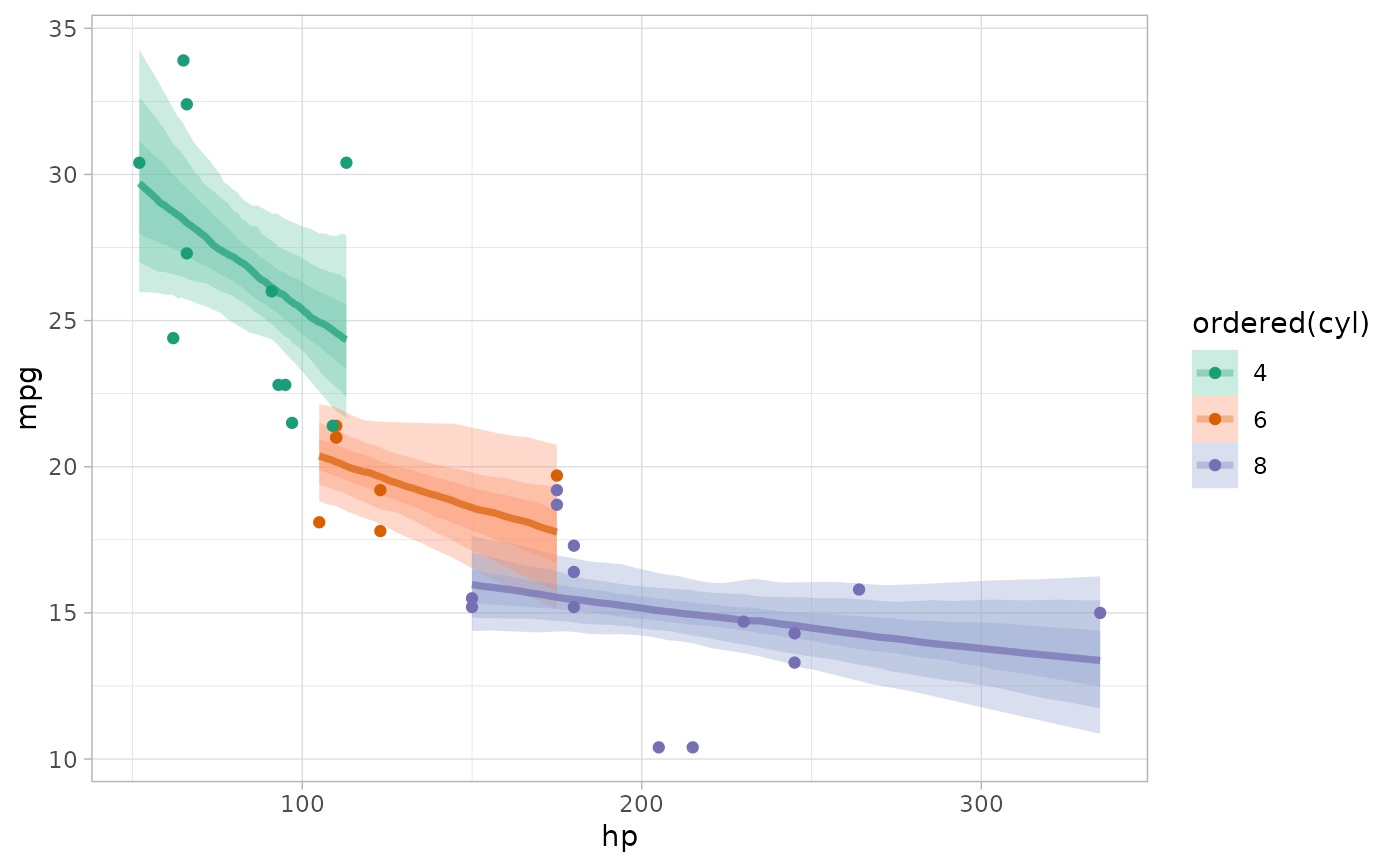
# plot intervals around conditional means (epred_rvars)
mtcars %>%
  group_by(cyl) %>%
  data_grid(hp = seq_range(hp, n = 101)) %>%
  add_epred_rvars(m_mpg) %>%
  ggplot(aes(x = hp, color = ordered(cyl), fill = ordered(cyl))) +
  stat_lineribbon(aes(dist = .epred), .width = c(.95, .8, .5), alpha = 1/3) +
  geom_point(aes(y = mpg), data = mtcars) +
  scale_color_brewer(palette = "Dark2") +
  scale_fill_brewer(palette = "Set2")


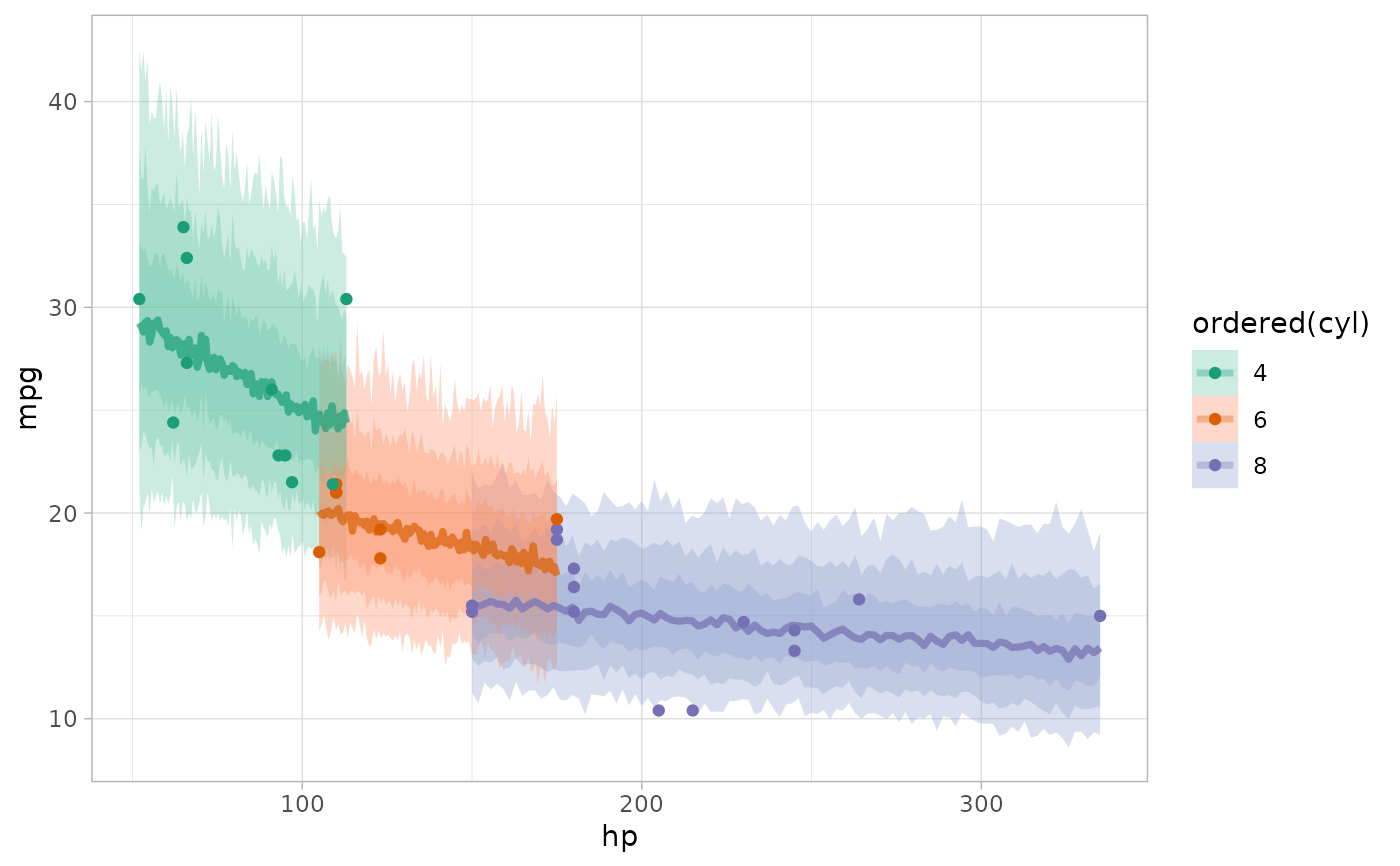
# plot posterior predictive intervals (predicted_rvars)
mtcars %>%
  group_by(cyl) %>%
  data_grid(hp = seq_range(hp, n = 101)) %>%
  add_predicted_rvars(m_mpg) %>%
  ggplot(aes(x = hp, color = ordered(cyl), fill = ordered(cyl))) +
  stat_lineribbon(aes(dist = .prediction), .width = c(.95, .8, .5), alpha = 1/3) +
  geom_point(aes(y = mpg), data = mtcars) +
  scale_color_brewer(palette = "Dark2") +
  scale_fill_brewer(palette = "Set2")


# }

Add `rvar`s for the linear predictor, posterior expectation, posterior predictive, or residuals of a model to a data frame

Arguments

Value

Details

See also

Author

Examples