Add draws from the posterior fit, predictions, or residuals of a model to a data frame
Source:R/epred_draws.R, R/linpred_draws.R, R/predicted_draws.R, and 1 more
add_predicted_draws.RdGiven a data frame and a model, adds draws from the linear/link-level predictor, the expectation of the posterior predictive, the posterior predictive, or the residuals of a model to the data frame in a long format.
add_epred_draws(
  newdata,
  object,
  ...,
  value = ".epred",
  ndraws = NULL,
  seed = NULL,
  re_formula = NULL,
  category = ".category",
  dpar = NULL
)

epred_draws(
  object,
  newdata,
  ...,
  value = ".epred",
  ndraws = NULL,
  seed = NULL,
  re_formula = NULL,
  category = ".category",
  dpar = NULL
)

# Default S3 method
epred_draws(
  object,
  newdata,
  ...,
  value = ".epred",
  seed = NULL,
  category = NULL
)

# S3 method for class 'stanreg'
epred_draws(
  object,
  newdata,
  ...,
  value = ".epred",
  ndraws = NULL,
  seed = NULL,
  re_formula = NULL,
  category = ".category",
  dpar = NULL
)

# S3 method for class 'brmsfit'
epred_draws(
  object,
  newdata,
  ...,
  value = ".epred",
  ndraws = NULL,
  seed = NULL,
  re_formula = NULL,
  category = ".category",
  dpar = NULL
)

add_linpred_draws(
  newdata,
  object,
  ...,
  value = ".linpred",
  ndraws = NULL,
  seed = NULL,
  re_formula = NULL,
  category = ".category",
  dpar = NULL,
  n
)

linpred_draws(
  object,
  newdata,
  ...,
  value = ".linpred",
  ndraws = NULL,
  seed = NULL,
  re_formula = NULL,
  category = ".category",
  dpar = NULL,
  n,
  scale
)

# Default S3 method
linpred_draws(
  object,
  newdata,
  ...,
  value = ".linpred",
  seed = NULL,
  category = NULL
)

# S3 method for class 'stanreg'
linpred_draws(
  object,
  newdata,
  ...,
  value = ".linpred",
  ndraws = NULL,
  seed = NULL,
  re_formula = NULL,
  category = ".category",
  dpar = NULL
)

# S3 method for class 'brmsfit'
linpred_draws(
  object,
  newdata,
  ...,
  value = ".linpred",
  ndraws = NULL,
  seed = NULL,
  re_formula = NULL,
  category = ".category",
  dpar = NULL
)

add_predicted_draws(
  newdata,
  object,
  ...,
  value = ".prediction",
  ndraws = NULL,
  seed = NULL,
  re_formula = NULL,
  category = ".category",
  n
)

predicted_draws(
  object,
  newdata,
  ...,
  value = ".prediction",
  ndraws = NULL,
  seed = NULL,
  re_formula = NULL,
  category = ".category",
  n,
  prediction
)

# Default S3 method
predicted_draws(
  object,
  newdata,
  ...,
  value = ".prediction",
  seed = NULL,
  category = ".category"
)

# S3 method for class 'stanreg'
predicted_draws(
  object,
  newdata,
  ...,
  value = ".prediction",
  ndraws = NULL,
  seed = NULL,
  re_formula = NULL,
  category = ".category"
)

# S3 method for class 'brmsfit'
predicted_draws(
  object,
  newdata,
  ...,
  value = ".prediction",
  ndraws = NULL,
  seed = NULL,
  re_formula = NULL,
  category = ".category"
)

add_residual_draws(
  newdata,
  object,
  ...,
  value = ".residual",
  ndraws = NULL,
  seed = NULL,
  re_formula = NULL,
  category = ".category",
  n
)

residual_draws(
  object,
  newdata,
  ...,
  value = ".residual",
  ndraws = NULL,
  seed = NULL,
  re_formula = NULL,
  category = ".category",
  n,
  residual
)

# Default S3 method
residual_draws(object, newdata, ...)

# S3 method for class 'brmsfit'
residual_draws(
  object,
  newdata,
  ...,
  value = ".residual",
  ndraws = NULL,
  seed = NULL,
  re_formula = NULL,
  category = ".category"
)
Arguments
- newdata
Data frame to generate predictions from.
- object
A supported Bayesian model fit that can provide fits and predictions. Supported models are listed in the second section of tidybayes-models: Models Supporting Prediction. While other functions in this package (like
spread_draws()) support a wider range of models, to work withadd_epred_draws(),add_predicted_draws(), etc. a model must provide an interface for generating predictions, thus more generic Bayesian modeling interfaces likerunjagsandrstanare not directly supported for these functions (only wrappers around those languages that provide predictions, likerstanarmandbrm, are supported here).- ...
Additional arguments passed to the underlying prediction method for the type of model given.
- value
The name of the output column:
for
[add_]epred_draws(), defaults to".epred".for
[add_]predicted_draws(), defaults to".prediction".for
[add_]linpred_draws(), defaults to".linpred".for
[add_]residual_draws(), defaults to".residual"
- ndraws
The number of draws to return, or
NULLto return all draws.- seed
A seed to use when subsampling draws (i.e. when
ndrawsis notNULL).- re_formula
formula containing group-level effects to be considered in the prediction. If
NULL(default), include all group-level effects; ifNA, include no group-level effects. Some model types (such as brms::brmsfit and rstanarm::stanreg-objects) allow marginalizing over grouping factors by specifying new levels of a factor innewdata. In the case ofbrms::brm(), you must also passallow_new_levels = TRUEhere to include new levels (seebrms::posterior_predict()).- category
For some ordinal, multinomial, and multivariate models (notably,
brms::brm()models but notrstanarm::stan_polr()models), multiple sets of rows will be returned per input row forepred_draws()orpredicted_draws(), depending on the model type. For ordinal/multinomial models, these rows correspond to different categories of the response variable. For multivariate models, these correspond to different response variables. Thecategoryargument specifies the name of the column to put the category names (or variable names) into in the resulting data frame. The default name of this column (".category") reflects the fact that this functionality was originally used only for ordinal models and has been re-used for multivariate models. The fact that multiple rows per response are returned only for some model types reflects the fact that tidybayes takes the approach of tidying whatever output is given to us, and the output from different modeling functions differs on this point. Seevignette("tidy-brms")andvignette("tidy-rstanarm")for examples of dealing with output from ordinal models using both approaches.- dpar
For
add_epred_draws()andadd_linpred_draws(): Should distributional regression parameters be included in the output? Valid only for models that support distributional regression parameters, such as submodels for variance parameters (as inbrms::brm()). IfTRUE, distributional regression parameters are included in the output as additional columns named after each parameter (alternative names can be provided using a list or named vector, e.g.c(sigma.hat = "sigma")would output the"sigma"parameter from a model as a column named"sigma.hat"). IfNULLorFALSE(the default), distributional regression parameters are not included.- n
(Deprecated). Use
ndraws.- scale
(Deprecated). Use the appropriate function (
epred_draws()orlinpred_draws()) depending on what type of distribution you want. Forlinpred_draws(), you may want thetransformargument. Seerstanarm::posterior_linpred()orbrms::posterior_linpred().- prediction, residual
(Deprecated). Use
value.
Value
A data frame (actually, a tibble) with a .row column (a
factor grouping rows from the input newdata), .chain column (the chain
each draw came from, or NA if the model does not provide chain information),
.iteration column (the iteration the draw came from, or NA if the model does
not provide iteration information), and a .draw column (a unique index corresponding to each draw
from the distribution). In addition, epred_draws includes a column with its name specified by
the epred argument (default ".epred"); linpred_draws includes a column with its name
specified by the linpred argument (default ".linpred"), and
predicted_draws contains a column with its name specified by the .prediction argument (default
".prediction"). For convenience, the resulting data frame comes grouped by the original input rows.
Details
Consider a model like:
$$\begin{array}{rcl} y &\sim& \textrm{SomeDist}(\theta_1, \theta_2)\\ f_1(\theta_1) &=& \alpha_1 + \beta_1 x\\ f_2(\theta_2) &=& \alpha_2 + \beta_2 x \end{array}$$
This model has:
an outcome variable, \(y\)
a response distribution, \(\textrm{SomeDist}\), having parameters \(\theta_1\) (with link function \(f_1\)) and \(\theta_2\) (with link function \(f_2\))
a single predictor, \(x\)
coefficients \(\alpha_1\), \(\beta_1\), \(\alpha_2\), and \(\beta_2\)
We fit this model to some observed data, \(y_\textrm{obs}\), and predictors,
\(x_\textrm{obs}\). Given new values of predictors, \(x_\textrm{new}\),
supplied in the data frame newdata, the functions for posterior draws are
defined as follows:
add_predicted_draws()adds draws from the posterior predictive distribution, \(p(y_\textrm{new} | x_\textrm{new}, y_\textrm{obs})\), to the data. It corresponds torstanarm::posterior_predict()orbrms::posterior_predict().add_epred_draws()adds draws from the expectation of the posterior predictive distribution, aka the conditional expectation, \(E(y_\textrm{new} | x_\textrm{new}, y_\textrm{obs})\), to the data. It corresponds torstanarm::posterior_epred()orbrms::posterior_epred(). Not all models support this function.add_linpred_draws()adds draws from the posterior linear predictors to the data. It corresponds torstanarm::posterior_linpred()orbrms::posterior_linpred(). Depending on the model type and additional parameters passed, this may be:The untransformed linear predictor, e.g. \(p(f_1(\theta_1) | x_\textrm{new}, y_\textrm{obs})\) = \(p(\alpha_1 + \beta_1 x_\textrm{new} | x_\textrm{new}, y_\textrm{obs})\). This is returned by
add_linpred_draws(transform = FALSE)for brms and rstanarm models. It is analogous totype = "link"inpredict.glm().The inverse-link transformed linear predictor, e.g. \(p(\theta_1 | x_\textrm{new}, y_\textrm{obs})\) = \(p(f_1^{-1}(\alpha_1 + \beta_1 x_\textrm{new}) | x_\textrm{new}, y_\textrm{obs})\). This is returned by
add_linpred_draws(transform = TRUE)for brms and rstanarm models. It is analogous totype = "response"inpredict.glm().
NOTE:
add_linpred_draws(transform = TRUE)andadd_epred_draws()may be equivalent but are not guaranteed to be. They are equivalent when the expectation of the response distribution is equal to its first parameter, i.e. when \(E(y) = \theta_1\). Many distributions have this property (e.g. Normal distributions, Bernoulli distributions), but not all. If you want the expectation of the posterior predictive, it is best to useadd_epred_draws()if available, and if not available, verify this property holds prior to usingadd_linpred_draws().add_residual_draws()adds draws from residuals, \(p(y_\textrm{obs} - y_\textrm{new} | x_\textrm{new}, y_\textrm{obs})\), to the data. It corresponds tobrms::residuals.brmsfit().
The corresponding functions without add_ as a prefix are alternate spellings
with the opposite order of the first two arguments: e.g. add_predicted_draws(newdata, object)
versus predicted_draws(object, newdata). This facilitates use in data
processing pipelines that start either with a data frame or a model.
Given equal choice between the two, the spellings prefixed with add_
are preferred.
See also
add_draws() for the variant of these functions for use with packages that do not have
explicit support for these functions yet. See spread_draws() for manipulating posteriors directly.
Examples
# \dontrun{
library(ggplot2)
library(dplyr)
library(brms)
library(modelr)
theme_set(theme_light())
m_mpg = brm(mpg ~ hp * cyl, data = mtcars,
# 1 chain / few iterations just so example runs quickly
# do not use in practice
chains = 1, iter = 500)
#> Compiling Stan program...
#> Start sampling
#>
#> SAMPLING FOR MODEL 'anon_model' NOW (CHAIN 1).
#> Chain 1:
#> Chain 1: Gradient evaluation took 4.3e-05 seconds
#> Chain 1: 1000 transitions using 10 leapfrog steps per transition would take 0.43 seconds.
#> Chain 1: Adjust your expectations accordingly!
#> Chain 1:
#> Chain 1:
#> Chain 1: Iteration: 1 / 500 [ 0%] (Warmup)
#> Chain 1: Iteration: 50 / 500 [ 10%] (Warmup)
#> Chain 1: Iteration: 100 / 500 [ 20%] (Warmup)
#> Chain 1: Iteration: 150 / 500 [ 30%] (Warmup)
#> Chain 1: Iteration: 200 / 500 [ 40%] (Warmup)
#> Chain 1: Iteration: 250 / 500 [ 50%] (Warmup)
#> Chain 1: Iteration: 251 / 500 [ 50%] (Sampling)
#> Chain 1: Iteration: 300 / 500 [ 60%] (Sampling)
#> Chain 1: Iteration: 350 / 500 [ 70%] (Sampling)
#> Chain 1: Iteration: 400 / 500 [ 80%] (Sampling)
#> Chain 1: Iteration: 450 / 500 [ 90%] (Sampling)
#> Chain 1: Iteration: 500 / 500 [100%] (Sampling)
#> Chain 1:
#> Chain 1: Elapsed Time: 0.123 seconds (Warm-up)
#> Chain 1: 0.047 seconds (Sampling)
#> Chain 1: 0.17 seconds (Total)
#> Chain 1:
#> Warning: Bulk Effective Samples Size (ESS) is too low, indicating posterior means and medians may be unreliable.
#> Running the chains for more iterations may help. See
#> https://mc-stan.org/misc/warnings.html#bulk-ess
#> Warning: Tail Effective Samples Size (ESS) is too low, indicating posterior variances and tail quantiles may be unreliable.
#> Running the chains for more iterations may help. See
#> https://mc-stan.org/misc/warnings.html#tail-ess
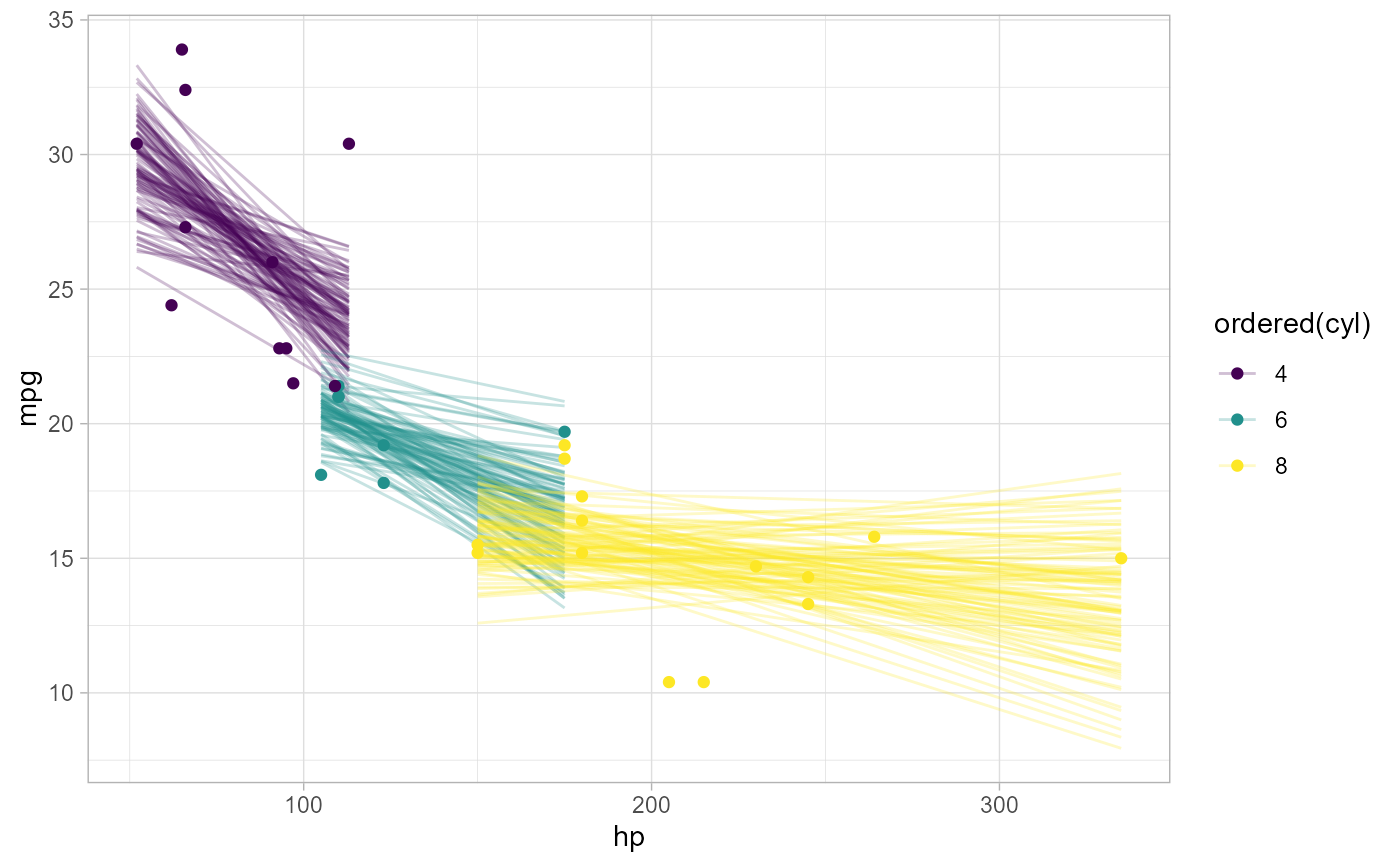
# draw 100 lines from the posterior means and overplot them
mtcars %>%
group_by(cyl) %>%
data_grid(hp = seq_range(hp, n = 101)) %>%
# NOTE: only use ndraws here when making spaghetti plots; for
# plotting intervals it is always best to use all draws (omit ndraws)
add_epred_draws(m_mpg, ndraws = 100) %>%
ggplot(aes(x = hp, y = mpg, color = ordered(cyl))) +
geom_line(aes(y = .epred, group = paste(cyl, .draw)), alpha = 0.25) +
geom_point(data = mtcars)
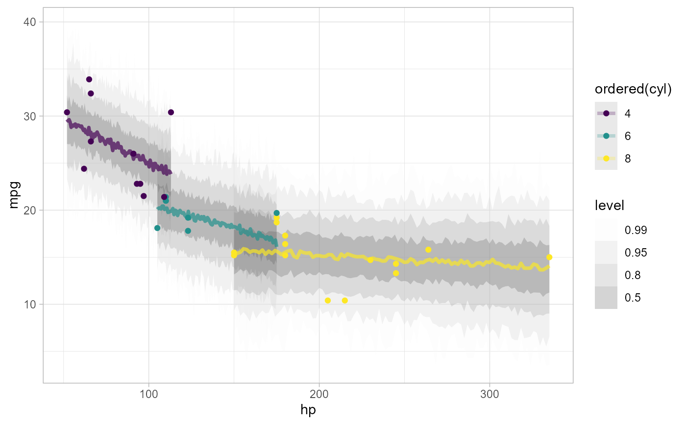
 # plot posterior predictive intervals
mtcars %>%
group_by(cyl) %>%
data_grid(hp = seq_range(hp, n = 101)) %>%
add_predicted_draws(m_mpg) %>%
ggplot(aes(x = hp, y = mpg, color = ordered(cyl))) +
stat_lineribbon(aes(y = .prediction), .width = c(.99, .95, .8, .5), alpha = 0.25) +
geom_point(data = mtcars) +
scale_fill_brewer(palette = "Greys")
# plot posterior predictive intervals
mtcars %>%
group_by(cyl) %>%
data_grid(hp = seq_range(hp, n = 101)) %>%
add_predicted_draws(m_mpg) %>%
ggplot(aes(x = hp, y = mpg, color = ordered(cyl))) +
stat_lineribbon(aes(y = .prediction), .width = c(.99, .95, .8, .5), alpha = 0.25) +
geom_point(data = mtcars) +
scale_fill_brewer(palette = "Greys")
 # }
# }