Turn tidy data frames of variables from a Bayesian model back into untidy data
Source:R/ungather_draws.R, R/unspread_draws.R
unspread_draws.RdInverse operations of spread_draws() and gather_draws(), giving
results that look like tidy_draws().
Arguments
- data
A tidy data frame of draws, such as one output by
spread_drawsorgather_draws.- ...
Expressions in the form of
variable_name[dimension_1, dimension_2, ...]. Seespread_draws().- variable
The name of the column in
datathat contains the names of variables from the model.- value
The name of the column in
datathat contains draws from the variables.- draw_indices
Character vector of column names that should be treated as indices of draws. Operations are done within combinations of these values. The default is
c(".chain", ".iteration", ".draw"), which is the same names used for chain, iteration, and draw indices returned bytidy_draws(). Names indraw_indicesthat are not found in the data are ignored.- drop_indices
Drop the columns specified by
draw_indicesfrom the resulting data frame. DefaultFALSE.
Value
A data frame.
Details
These functions take symbolic specifications of variable names and dimensions in the same format as
spread_draws() and gather_draws() and invert the tidy data frame back into
a data frame whose column names are variables with dimensions in them.
See also
Examples
library(dplyr)

data(RankCorr, package = "ggdist")

# We can use unspread_draws to allow us to manipulate draws with tidybayes
# and then transform the draws into a form we can use with packages like bayesplot.
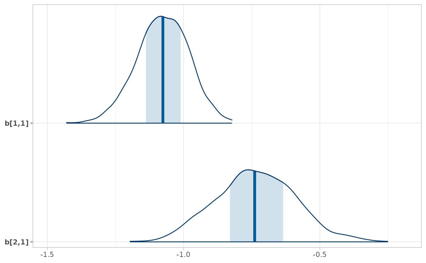
# Here we subset b[i,j] to just values of i in 1:2 and j == 1, then plot with bayesplot
RankCorr %>%
  spread_draws(b[i,j]) %>%
  filter(i %in% 1:2, j == 1) %>%
  unspread_draws(b[i,j], drop_indices = TRUE) %>%
  bayesplot::mcmc_areas()


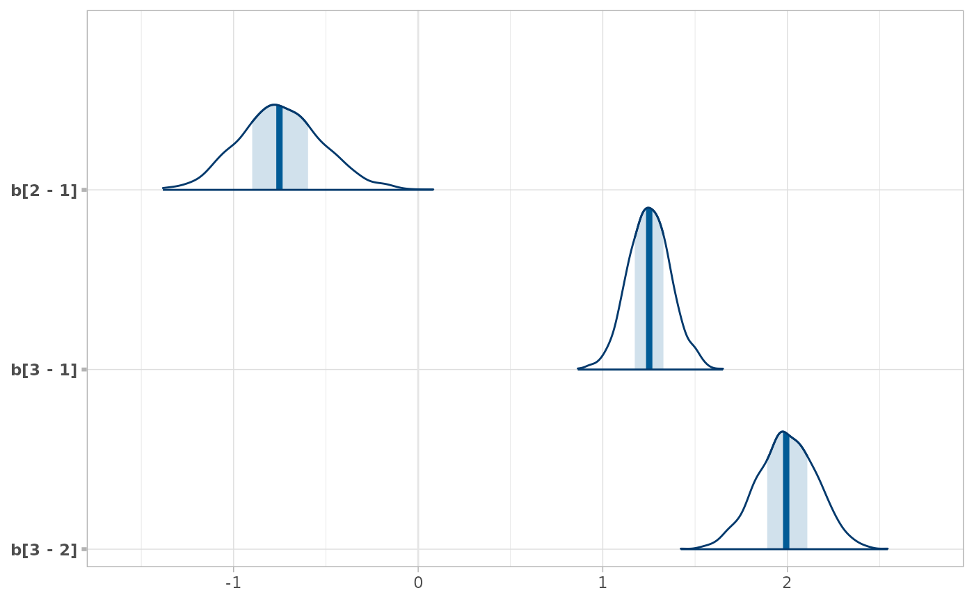
# As another example, we could use compare_levels to plot all pairwise comparisons
# of b[1,j] for j in 1:3
RankCorr %>%
  spread_draws(b[i,j]) %>%
  filter(i == 1, j %in% 1:3) %>%
  compare_levels(b, by = j) %>%
  unspread_draws(b[j], drop_indices = TRUE) %>%
  bayesplot::mcmc_areas()
