Density bins and histogram bins as data frames

Generates a data frame of bins representing the kernel density (or histogram) of a vector, suitable for use in generating predictive distributions for visualization. These functions were originally designed for use with the now-deprecated predict_curve(), and may be deprecated in the future.

density_bins(x, n = 101, ...)

histogram_bins(x, n = 30, breaks = n, ...)

Arguments

x: A numeric vector
n: Number of bins
...: Additional arguments passed to density() or hist().
breaks: Used to set bins for histogram_bins. Can be number of bins (by default it is set to the value of n) or a method for setting bins. See the breaks argument of hist().

Value

A data frame representing bins and their densities with the following columns:

mid: Bin midpoint
lower: Lower endpoint of each bin
upper: Upper endpoint of each bin
density: Density estimate of the bin

Details

These functions are simple wrappers to density() and hist() that compute density estimates and return their results in a consistent format: a data frame of bins suitable for use with the now-deprecated predict_curve().

density_bins computes a kernel density estimate using density().

histogram_bins computes a density histogram using hist().

Author

Matthew Kay

Examples

# \dontrun{

library(ggplot2)
library(dplyr)
library(brms)
library(modelr)

theme_set(theme_light())

m_mpg = brm(mpg ~ hp * cyl, data = mtcars)
#> Compiling Stan program...
#> Start sampling
#> 
#> SAMPLING FOR MODEL 'anon_model' NOW (CHAIN 1).
#> Chain 1: 
#> Chain 1: Gradient evaluation took 5.8e-05 seconds
#> Chain 1: 1000 transitions using 10 leapfrog steps per transition would take 0.58 seconds.
#> Chain 1: Adjust your expectations accordingly!
#> Chain 1: 
#> Chain 1: 
#> Chain 1: Iteration:    1 / 2000 [  0%]  (Warmup)
#> Chain 1: Iteration:  200 / 2000 [ 10%]  (Warmup)
#> Chain 1: Iteration:  400 / 2000 [ 20%]  (Warmup)
#> Chain 1: Iteration:  600 / 2000 [ 30%]  (Warmup)
#> Chain 1: Iteration:  800 / 2000 [ 40%]  (Warmup)
#> Chain 1: Iteration: 1000 / 2000 [ 50%]  (Warmup)
#> Chain 1: Iteration: 1001 / 2000 [ 50%]  (Sampling)
#> Chain 1: Iteration: 1200 / 2000 [ 60%]  (Sampling)
#> Chain 1: Iteration: 1400 / 2000 [ 70%]  (Sampling)
#> Chain 1: Iteration: 1600 / 2000 [ 80%]  (Sampling)
#> Chain 1: Iteration: 1800 / 2000 [ 90%]  (Sampling)
#> Chain 1: Iteration: 2000 / 2000 [100%]  (Sampling)
#> Chain 1: 
#> Chain 1:  Elapsed Time: 0.34 seconds (Warm-up)
#> Chain 1:                0.175 seconds (Sampling)
#> Chain 1:                0.515 seconds (Total)
#> Chain 1: 
#> 
#> SAMPLING FOR MODEL 'anon_model' NOW (CHAIN 2).
#> Chain 2: 
#> Chain 2: Gradient evaluation took 6e-06 seconds
#> Chain 2: 1000 transitions using 10 leapfrog steps per transition would take 0.06 seconds.
#> Chain 2: Adjust your expectations accordingly!
#> Chain 2: 
#> Chain 2: 
#> Chain 2: Iteration:    1 / 2000 [  0%]  (Warmup)
#> Chain 2: Iteration:  200 / 2000 [ 10%]  (Warmup)
#> Chain 2: Iteration:  400 / 2000 [ 20%]  (Warmup)
#> Chain 2: Iteration:  600 / 2000 [ 30%]  (Warmup)
#> Chain 2: Iteration:  800 / 2000 [ 40%]  (Warmup)
#> Chain 2: Iteration: 1000 / 2000 [ 50%]  (Warmup)
#> Chain 2: Iteration: 1001 / 2000 [ 50%]  (Sampling)
#> Chain 2: Iteration: 1200 / 2000 [ 60%]  (Sampling)
#> Chain 2: Iteration: 1400 / 2000 [ 70%]  (Sampling)
#> Chain 2: Iteration: 1600 / 2000 [ 80%]  (Sampling)
#> Chain 2: Iteration: 1800 / 2000 [ 90%]  (Sampling)
#> Chain 2: Iteration: 2000 / 2000 [100%]  (Sampling)
#> Chain 2: 
#> Chain 2:  Elapsed Time: 0.318 seconds (Warm-up)
#> Chain 2:                0.132 seconds (Sampling)
#> Chain 2:                0.45 seconds (Total)
#> Chain 2: 
#> 
#> SAMPLING FOR MODEL 'anon_model' NOW (CHAIN 3).
#> Chain 3: 
#> Chain 3: Gradient evaluation took 7e-06 seconds
#> Chain 3: 1000 transitions using 10 leapfrog steps per transition would take 0.07 seconds.
#> Chain 3: Adjust your expectations accordingly!
#> Chain 3: 
#> Chain 3: 
#> Chain 3: Iteration:    1 / 2000 [  0%]  (Warmup)
#> Chain 3: Iteration:  200 / 2000 [ 10%]  (Warmup)
#> Chain 3: Iteration:  400 / 2000 [ 20%]  (Warmup)
#> Chain 3: Iteration:  600 / 2000 [ 30%]  (Warmup)
#> Chain 3: Iteration:  800 / 2000 [ 40%]  (Warmup)
#> Chain 3: Iteration: 1000 / 2000 [ 50%]  (Warmup)
#> Chain 3: Iteration: 1001 / 2000 [ 50%]  (Sampling)
#> Chain 3: Iteration: 1200 / 2000 [ 60%]  (Sampling)
#> Chain 3: Iteration: 1400 / 2000 [ 70%]  (Sampling)
#> Chain 3: Iteration: 1600 / 2000 [ 80%]  (Sampling)
#> Chain 3: Iteration: 1800 / 2000 [ 90%]  (Sampling)
#> Chain 3: Iteration: 2000 / 2000 [100%]  (Sampling)
#> Chain 3: 
#> Chain 3:  Elapsed Time: 0.318 seconds (Warm-up)
#> Chain 3:                0.194 seconds (Sampling)
#> Chain 3:                0.512 seconds (Total)
#> Chain 3: 
#> 
#> SAMPLING FOR MODEL 'anon_model' NOW (CHAIN 4).
#> Chain 4: 
#> Chain 4: Gradient evaluation took 6e-06 seconds
#> Chain 4: 1000 transitions using 10 leapfrog steps per transition would take 0.06 seconds.
#> Chain 4: Adjust your expectations accordingly!
#> Chain 4: 
#> Chain 4: 
#> Chain 4: Iteration:    1 / 2000 [  0%]  (Warmup)
#> Chain 4: Iteration:  200 / 2000 [ 10%]  (Warmup)
#> Chain 4: Iteration:  400 / 2000 [ 20%]  (Warmup)
#> Chain 4: Iteration:  600 / 2000 [ 30%]  (Warmup)
#> Chain 4: Iteration:  800 / 2000 [ 40%]  (Warmup)
#> Chain 4: Iteration: 1000 / 2000 [ 50%]  (Warmup)
#> Chain 4: Iteration: 1001 / 2000 [ 50%]  (Sampling)
#> Chain 4: Iteration: 1200 / 2000 [ 60%]  (Sampling)
#> Chain 4: Iteration: 1400 / 2000 [ 70%]  (Sampling)
#> Chain 4: Iteration: 1600 / 2000 [ 80%]  (Sampling)
#> Chain 4: Iteration: 1800 / 2000 [ 90%]  (Sampling)
#> Chain 4: Iteration: 2000 / 2000 [100%]  (Sampling)
#> Chain 4: 
#> Chain 4:  Elapsed Time: 0.257 seconds (Warm-up)
#> Chain 4:                0.139 seconds (Sampling)
#> Chain 4:                0.396 seconds (Total)
#> Chain 4: 

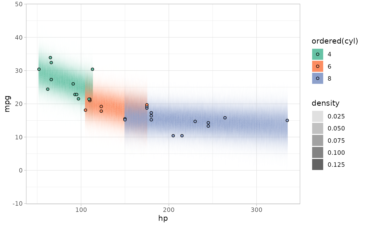
step = 1
mtcars %>%
  group_by(cyl) %>%
  data_grid(hp = seq_range(hp, by = step)) %>%
  add_predicted_draws(m_mpg) %>%
  summarise(density_bins(.prediction), .groups = "drop") %>%
  ggplot() +
  geom_rect(aes(
    xmin = hp - step/2, ymin = lower, ymax = upper, xmax = hp + step/2,
    fill = ordered(cyl), alpha = density
  )) +
  geom_point(aes(x = hp, y = mpg, fill = ordered(cyl)), shape = 21, data = mtcars) +
  scale_alpha_continuous(range = c(0, 1)) +
  scale_fill_brewer(palette = "Set2")
#> Warning: Returning more (or less) than 1 row per `summarise()` group was deprecated in
#> dplyr 1.1.0.
#> ℹ Please use `reframe()` instead.
#> ℹ When switching from `summarise()` to `reframe()`, remember that `reframe()`
#>   always returns an ungrouped data frame and adjust accordingly.


# }

Arguments

Value

Details

See also

Author

Examples