Point and interval summaries for tidy data frames of draws from distributions

Translates draws from distributions in a (possibly grouped) data frame into point and interval summaries (or set of point and interval summaries, if there are multiple groups in a grouped data frame).

Usage

point_interval(
  .data,
  ...,
  .width = 0.95,
  .point = median,
  .interval = qi,
  .simple_names = TRUE,
  na.rm = FALSE,
  .exclude = c(".chain", ".iteration", ".draw", ".row"),
  .prob
)

# S3 method for default
point_interval(
  .data,
  ...,
  .width = 0.95,
  .point = median,
  .interval = qi,
  .simple_names = TRUE,
  na.rm = FALSE,
  .exclude = c(".chain", ".iteration", ".draw", ".row"),
  .prob
)

# S3 method for numeric
point_interval(
  .data,
  ...,
  .width = 0.95,
  .point = median,
  .interval = qi,
  .simple_names = FALSE,
  na.rm = FALSE,
  .exclude = c(".chain", ".iteration", ".draw", ".row"),
  .prob
)

# S3 method for rvar
point_interval(
  .data,
  ...,
  .width = 0.95,
  .point = median,
  .interval = qi,
  .simple_names = TRUE,
  na.rm = FALSE
)

# S3 method for distribution
point_interval(
  .data,
  ...,
  .width = 0.95,
  .point = median,
  .interval = qi,
  .simple_names = TRUE,
  na.rm = FALSE
)

qi(x, .width = 0.95, .prob, na.rm = FALSE)

ll(x, .width = 0.95, na.rm = FALSE)

ul(x, .width = 0.95, na.rm = FALSE)

hdi(
  x,
  .width = 0.95,
  na.rm = FALSE,
  ...,
  density = density_bounded(trim = TRUE),
  n = 4096,
  .prob
)

Mode(x, na.rm = FALSE, ...)

# S3 method for default
Mode(
  x,
  na.rm = FALSE,
  ...,
  density = density_bounded(trim = TRUE),
  n = 2001,
  weights = NULL
)

# S3 method for rvar
Mode(x, na.rm = FALSE, ...)

# S3 method for distribution
Mode(x, na.rm = FALSE, ...)

hdci(x, .width = 0.95, na.rm = FALSE)

mean_qi(.data, ..., .width = 0.95)

median_qi(.data, ..., .width = 0.95)

mode_qi(.data, ..., .width = 0.95)

mean_ll(.data, ..., .width = 0.95)

median_ll(.data, ..., .width = 0.95)

mode_ll(.data, ..., .width = 0.95)

mean_ul(.data, ..., .width = 0.95)

median_ul(.data, ..., .width = 0.95)

mode_ul(.data, ..., .width = 0.95)

mean_hdi(.data, ..., .width = 0.95)

median_hdi(.data, ..., .width = 0.95)

mode_hdi(.data, ..., .width = 0.95)

mean_hdci(.data, ..., .width = 0.95)

median_hdci(.data, ..., .width = 0.95)

mode_hdci(.data, ..., .width = 0.95)

Arguments

.data: Data frame (or grouped data frame as returned by dplyr::group_by()) that contains draws to summarize.
...: Bare column names or expressions that, when evaluated in the context of .data, represent draws to summarize. If this is empty, then by default all columns that are not group columns and which are not in .exclude (by default ".chain", ".iteration", ".draw", and ".row") will be summarized. These columns can be numeric, distributional objects, posterior::rvars, or list columns of numeric values to summarise.
.width: vector of probabilities to use that determine the widths of the resulting intervals. If multiple probabilities are provided, multiple rows per group are generated, each with a different probability interval (and value of the corresponding .width column).
.point: Point summary function, which takes a vector and returns a single value, e.g. mean(), median(), or Mode().
.interval: Interval function, which takes a vector and a probability (.width) and returns a two-element vector representing the lower and upper bound of an interval; e.g. qi(), hdi()
.simple_names: When TRUE and only a single column / vector is to be summarized, use the name .lower for the lower end of the interval and .upper for the upper end. If .data is a vector and this is TRUE, this will also set the column name of the point summary to .value. When FALSE and .data is a data frame, names the lower and upper intervals for each column x x.lower and x.upper. When FALSE and .data is a vector, uses the naming scheme y, ymin and ymax (for use with ggplot).
na.rm: logical value indicating whether NA values should be stripped before the computation proceeds. If FALSE (the default), any vectors to be summarized that contain NA will result in point and interval summaries equal to NA.
.exclude: A character vector of names of columns to be excluded from summarization if no column names are specified to be summarized. Default ignores several meta-data column names used in ggdist and tidybayes.
.prob: Deprecated. Use .width instead.
x: vector to summarize (for interval functions: qi and hdi)
density: For hdi() and Mode(), the kernel density estimator to use, either as a function (e.g. density_bounded, density_unbounded) or as a string giving the suffix to a function that starts with density_ (e.g. "bounded" or "unbounded"). The default, "bounded", uses the bounded density estimator of density_bounded(), which itself estimates the bounds of the distribution, and tends to work well on both bounded and unbounded data.
n: For hdi() and Mode(), the number of points to use to estimate highest-density intervals or modes.
weights: For Mode(), an optional vector, which (if not NULL) is of the same length as x and provides weights for each element of x.

Value

A data frame containing point summaries and intervals, with at least one column corresponding to the point summary, one to the lower end of the interval, one to the upper end of the interval, the width of the interval (.width), the type of point summary (.point), and the type of interval (.interval).

Details

If .data is a data frame, then ... is a list of bare names of columns (or expressions derived from columns) of .data, on which the point and interval summaries are derived. Column expressions are processed using the tidy evaluation framework (see rlang::eval_tidy()).

For a column named x, the resulting data frame will have a column named x containing its point summary. If there is a single column to be summarized and .simple_names is TRUE, the output will also contain columns .lower (the lower end of the interval), .upper (the upper end of the interval). Otherwise, for every summarized column x, the output will contain x.lower (the lower end of the interval) and x.upper (the upper end of the interval). Finally, the output will have a .width column containing the' probability for the interval on each output row.

If .data includes groups (see e.g. dplyr::group_by()), the points and intervals are calculated within the groups.

If .data is a vector, ... is ignored and the result is a data frame with one row per value of .width and three columns: y (the point summary), ymin (the lower end of the interval), ymax (the upper end of the interval), and .width, the probability corresponding to the interval. This behavior allows point_interval and its derived functions (like median_qi, mean_qi, mode_hdi, etc) to be easily used to plot intervals in ggplot stats using methods like stat_eye(), stat_halfeye(), or stat_summary().

median_qi, mode_hdi, etc are short forms for point_interval(..., .point = median, .interval = qi), etc.

qi yields the quantile interval (also known as the percentile interval or equi-tailed interval) as a 1x2 matrix.

hdi yields the highest-density interval(s) (also known as the highest posterior density interval). Note: If the distribution is multimodal, hdi may return multiple intervals for each probability level (these will be spread over rows). You may wish to use hdci (below) instead if you want a single highest-density interval, with the caveat that when the distribution is multimodal hdci is not a highest-density interval.

hdci yields the highest-density continuous interval, also known as the shortest probability interval. Note: If the distribution is multimodal, this may not actually be the highest-density interval (there may be a higher-density discontinuous interval, which can be found using hdi).

ll and ul yield lower limits and upper limits, respectively (where the opposite limit is set to either Inf or -Inf).

Author

Matthew Kay

Examples


library(dplyr)
library(ggplot2)

set.seed(123)

rnorm(1000) %>%
  median_qi()
#>             y      ymin     ymax .width .point .interval
#> 1 0.009209639 -1.941554 2.037887   0.95 median        qi

data.frame(x = rnorm(1000)) %>%
  median_qi(x, .width = c(.50, .80, .95))
#> # A tibble: 3 × 6
#>        x .lower .upper .width .point .interval
#>    <dbl>  <dbl>  <dbl>  <dbl> <chr>  <chr>    
#> 1 0.0549 -0.653  0.753   0.5  median qi       
#> 2 0.0549 -1.24   1.34    0.8  median qi       
#> 3 0.0549 -1.99   1.91    0.95 median qi       

data.frame(
    x = rnorm(1000),
    y = rnorm(1000, mean = 2, sd = 2)
  ) %>%
  median_qi(x, y)
#>             x   x.lower  x.upper        y   y.lower  y.upper .width .point
#> 1 -0.05057431 -2.012529 1.934141 1.983618 -1.946229 5.947635   0.95 median
#>   .interval
#> 1        qi

data.frame(
    x = rnorm(1000),
    group = "a"
  ) %>%
  rbind(data.frame(
    x = rnorm(1000, mean = 2, sd = 2),
    group = "b")
  ) %>%
  group_by(group) %>%
  median_qi(.width = c(.50, .80, .95))
#> # A tibble: 6 × 7
#>   group       x .lower .upper .width .point .interval
#>   <chr>   <dbl>  <dbl>  <dbl>  <dbl> <chr>  <chr>    
#> 1 a     -0.0328 -0.707  0.636   0.5  median qi       
#> 2 b      2.06    0.759  3.44    0.5  median qi       
#> 3 a     -0.0328 -1.27   1.23    0.8  median qi       
#> 4 b      2.06   -0.559  4.48    0.8  median qi       
#> 5 a     -0.0328 -2.00   1.84    0.95 median qi       
#> 6 b      2.06   -1.75   5.91    0.95 median qi       

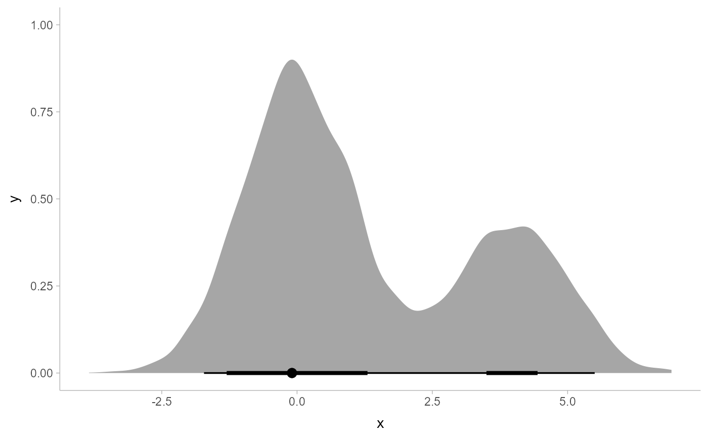
multimodal_draws = data.frame(
    x = c(rnorm(5000, 0, 1), rnorm(2500, 4, 1))
  )

multimodal_draws %>%
  mode_hdi(.width = c(.66, .95))
#> # A tibble: 3 × 6
#>         x .lower .upper .width .point .interval
#>     <dbl>  <dbl>  <dbl>  <dbl> <chr>  <chr>    
#> 1 -0.0938  -1.30   1.30   0.66 mode   hdi      
#> 2 -0.0938   3.50   4.44   0.66 mode   hdi      
#> 3 -0.0938  -1.72   5.50   0.95 mode   hdi      

multimodal_draws %>%
  ggplot(aes(x = x, y = 0)) +
  stat_halfeye(point_interval = mode_hdi, .width = c(.66, .95))